Chapter 17 Prediction from the linear model
17.1 Introduction
One use of a regression model is prediction. That is, the model is used to predict, or estimate, values of the response \(y\) given values of the explanatory variables \(x\). This could involve interpolation (e.g. estimating \(y\) within the known range of \(x\)) or extrapolation (e.g. estimating \(y\) outwith the known range of \(x\), or combination of \(x\)’s in multiple regression). As well as estimating a particular value (point estimate), we also need to provide a measure of uncertainty of the estimate and this will depend on the aim of the prediction.
In this chapter, we illustrate how to obtain a predicted value and the associated uncertainty.
17.2 Prediction
Imagine a regression of height (explanatory variable) and IQ (response) amongst a sample of humans (Figure 17.1). These data are stored in a dataframe df1 and a simple linear regression model has been fitted (a summary is given below):
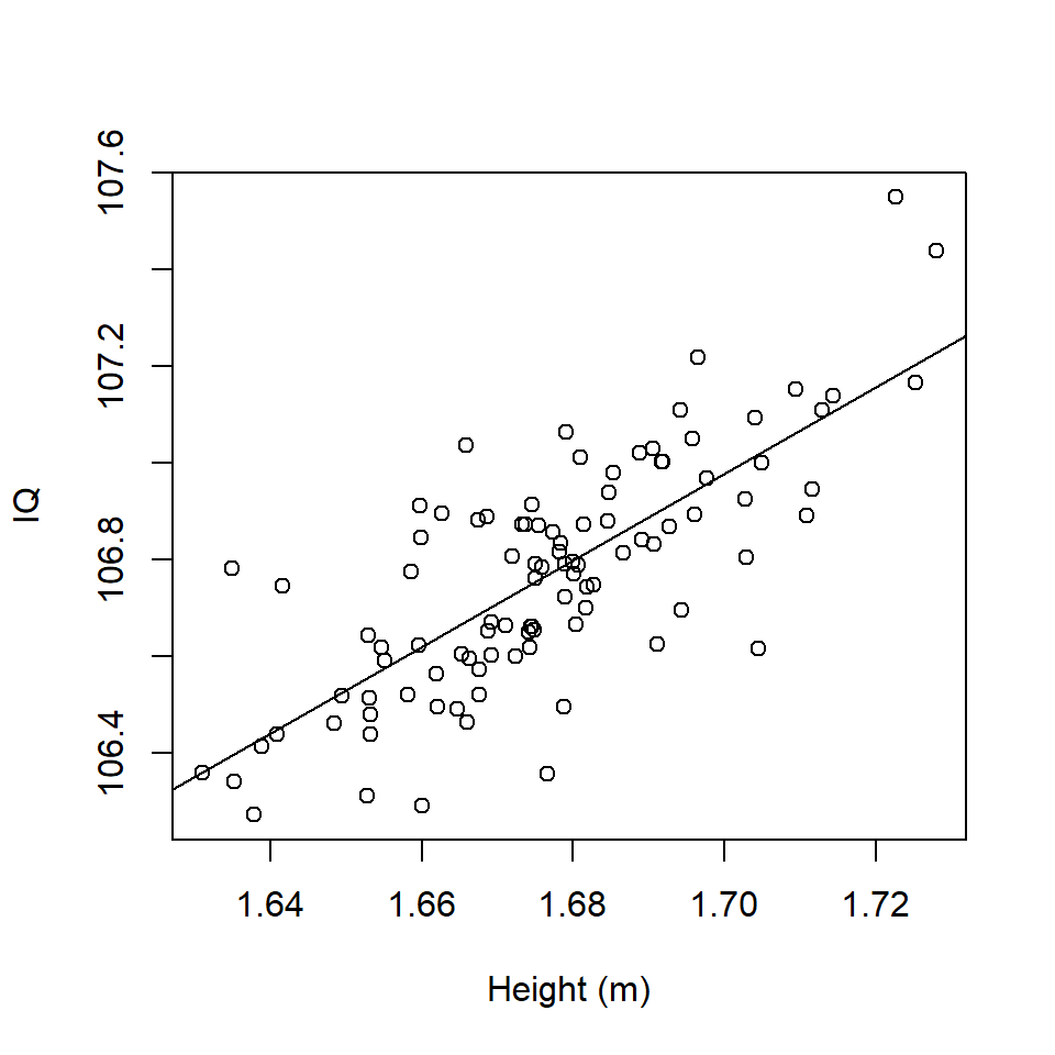
Figure 17.1: Scatterplot of Height (m) and IQ and fitted regression line.
# Fit model
modelIQ <- lm(IQ ~ Height, data=df1)
# Summary
summary(modelIQ)
Call:
lm(formula = IQ ~ Height, data = df1)

Residuals:
     Min       1Q   Median       3Q      Max
-0.41039 -0.08653 -0.01571  0.09717  0.38772

Coefficients:
            Estimate Std. Error t value Pr(>|t|)
(Intercept)  91.7687     1.3090   70.11   <2e-16 ***
Height        8.9463     0.7807   11.46   <2e-16 ***
---
Signif. codes:  0 '***' 0.001 '**' 0.01 '*' 0.05 '.' 0.1 ' ' 1

Residual standard error: 0.1586 on 98 degrees of freedom
Multiple R-squared:  0.5726,    Adjusted R-squared:  0.5683
F-statistic: 131.3 on 1 and 98 DF,  p-value: < 2.2e-16
# ANOVA
anova(modelIQ)Analysis of Variance Table
Response: IQ
Df Sum Sq Mean Sq F value Pr(>F)
Height 1 3.3021 3.3021 131.31 < 2.2e-16 ***
Residuals 98 2.4645 0.0251
---
Signif. codes: 0 '***' 0.001 '**' 0.01 '*' 0.05 '.' 0.1 ' ' 1From the model summary, the fitted equation from this model is: \[\hat {\textrm{IQ}} = 91.769+8.946 \times \textrm{Height}\] If we wanted to obtain the estimate of IQ for a height of 1.72m, then the point estimate is given by:
\[\hat {\textrm{IQ}} =91.769 + 8.946 \times 1.72 = 107.156\]
This predicted value is the black cross in Figure 17.2.

Figure 17.2: Scatterplot of Height (m) and IQ with a predicted value (black cross).
17.2.1 Doing this in R
We can (moderately) easily do the prediction in R by creating a new data frame containing the values we want predictions for and then use the predict function:
# Specify value for height
Height <- 1.72
# Create data frame
df2 <- data.frame(Height)
# Prediction using specified linear model object
predict(modelIQ, newdata=df2)
1
107.1563 Note that the name of the explanatory variable we wish to predict over in df2 (i.e. Height) has to match the name of the explanatory variable in the model object modelIQ.
17.3 Uncertainty in the prediction
As you have seen, getting a predicted value (point estimate) is simply a matter of substituting in for the relevant predictor variables, but it is also essential to obtain a measure of uncertainty. As usual, a standard error is required for the predicted value (denoted by \(\hat y_p\)):
\[se(\hat{y}_p)=\sqrt{MSE\times (\frac{1}{n}+\frac{(x_p-\bar{x})^2}{\sum{(x_i-\bar{x})^2}}})\] where
- \(MSE\) is the mean square error, or the residual, which can be obtained from the ANOVA table or the square of the residual standard error given by
summary - \(n\) is the number of observations
- \(x_p\) is the \(x\) value you want to predict on,
- \(i = 1, ..., n\)
- \(\bar x\) is the mean value of \(x\)
Then the confidence interval can be obtained as you have seen before:
\[\hat y_p \pm t_{(\alpha/2, df)}\times se(\hat{y}_p)\] where the \(t\) multiplier is found from the t distribution which has the relevant error degrees of freedom associated with the model.
We can now construct a 99% confidence interval for the mean response using the following components:
The mean square error is the square of the residual standard error, hence, \(MSE = 0.1586^2 = 0.0252\). The \(MSE\) is also provided in the ANOVA table.
Number of observations, \(n=100\)
Mean height is \(\bar{\mathrm{Height}}=1.676458\)
mean(df1$Height)[1] 1.676458- The sum of the difference between each value and the mean is given by
\[\sum{(\mathrm{Height}_i-\bar{\mathrm{Height}})^2} \]
sum((df1$Height - mean(df1$Height))^2)[1] 0.04125725Hence, the standard error is
\[se(\hat{IQ})=\sqrt{0.0252\times (\frac{1}{100}+\frac{(1.72-1.676)^2}{0.041})} =0.038\]
To obtain the confidence interval, we also need the relevant quantile for the 99% confidence interval. This is obtained from the \(t\) distribution where the degrees of freedom are associated with the error (residuals) term, i.e. \(df=98\).
# Want quantile with 0.5% in each tail
qt(p=0.005, df=98)[1] -2.626931Therefore, the CI is given by:
\[107.156 \pm -2.63\times 0.038\]
Lower bound: 107.058; Upper bound: 107.254
Thus, for a height of 1.72m, the predicted IQ is 107.156 (99% CI 107.01 - 107.25). In other words 99 out of 100 times a regression line was fitted to random data from this population the estimated mean IQ for a height of 1.72m would lie in the range 107.01 - 107.25.
17.3.1 Doing this in R
As usual this can be done simply in R, by adding the interval argument to the predict function.
# Prediction with CI
predict(modelIQ, newdata=df2, se.fit=TRUE, interval="confidence",
level=0.99)$fit
fit lwr upr
1 107.1563 107.0578 107.2549
$se.fit
[1] 0.03751133
$df
[1] 98
$residual.scale
[1] 0.1585812The “residual scale” here is, confusingly, the square of the mean square error.
17.3.2 Confidence intervals for the line
We can estimate the confidence interval for the whole line by supplying a range of predictor values to predict over:
# Obtain a sequence of Heights from min to max
Height <- seq(from=min(df1$Height), to=max(df1$Height), by=0.001)
Height[1:5]
[1] 1.630961 1.631961 1.632961 1.633961 1.634961# Create dataframe
df3 <- data.frame(Height)
# Prediction with CI
bounds.ci <- predict(modelIQ, newdata=df3, se.fit=T,
interval="confidence", level=0.99)
# Plot data
plot (df1$Height, df1$IQ, xlab="Height", ylab="IQ")
# Add regression line
abline (modelIQ)
# Add CI
lines (df3$Height, bounds.ci$fit[,3], lty=2)
lines (df3$Height, bounds.ci$fit[,2], lty=2)
Figure 17.3: Scatterplot of Height and IQ with confidence interval
This confidence interval (Figure 17.3) on the mean response is narrowest around mean value for Height (i.e. 1.676m) and the mean value of IQ (i.e. 106.8), \(pt(\bar{\mathrm{Height}},\bar{IQ})\). It is the confidence interval for the mean response, i.e. the overall uncertainty in the fit in the line.
17.3.3 Prediction intervals
Sometimes we are interested in the uncertainty in the individual predictions i.e. what range of values would we find in IQ for a man of height 1.72m. Not the mean response but the range of individual values that might plausibly be found. This is called a prediction interval as opposed to the confidence interval and is calculated as before, except with a slightly different estimate of standard error:
\[\textrm{prediction }se(\hat{y})=\sqrt{MSE\times (1+\frac{1}{n}+\frac{(x_p-\bar{x})^2}{\sum{(x_i-\bar{x})^2}})}\]
The prediction standard error for an observation at 1.72m is:
\[\textrm{prediction }se(\hat{IQ})=\sqrt{0.025\times (1+ \frac{1}{100}+\frac{(1.72-1.676)^2}{0.041})} =0.163\]
Hence, the 99% prediction interval for the response at 1.72m is:
\[107.156 \pm -2.63\times 0.163\]
Lower bound: 106.728
Upper bound: 107.585
17.3.3.1 Doing this in R
As before, we can use R to do things easily:
# Prediction CI
predict(modelIQ, newdata=df2, se.fit=TRUE, interval="prediction",
        level=0.99)
$fit
fit lwr upr
1 107.1563 106.7283 107.5844
$se.fit
[1] 0.03751133
$df
[1] 98
$residual.scale
[1] 0.1585812NB R still gives the confidence standard error.
And as before we can also construct a prediction interval over the entire range of heights. However this does not reflect the uncertainty in the mean response but the uncertainty in individual responses.
# Plot data
plot (df1$Height, df1$IQ, xlab="Height", ylab="IQ", ylim=c(105.9,107.6))
# Add regression line
abline (modelIQ)
# Add confidence interval
lines (Height, bounds.ci$fit[,3], lty=2)
lines (Height, bounds.ci$fit[,2], lty=2)
# Obtain prediction interval and add to plot
bounds.pi <- predict(modelIQ, newdata=df3, se.fit=TRUE,
                     interval="prediction", level=0.99)
lines (Height, bounds.pi$fit[,3], lty=3)
lines (Height, bounds.pi$fit[,2], lty=3)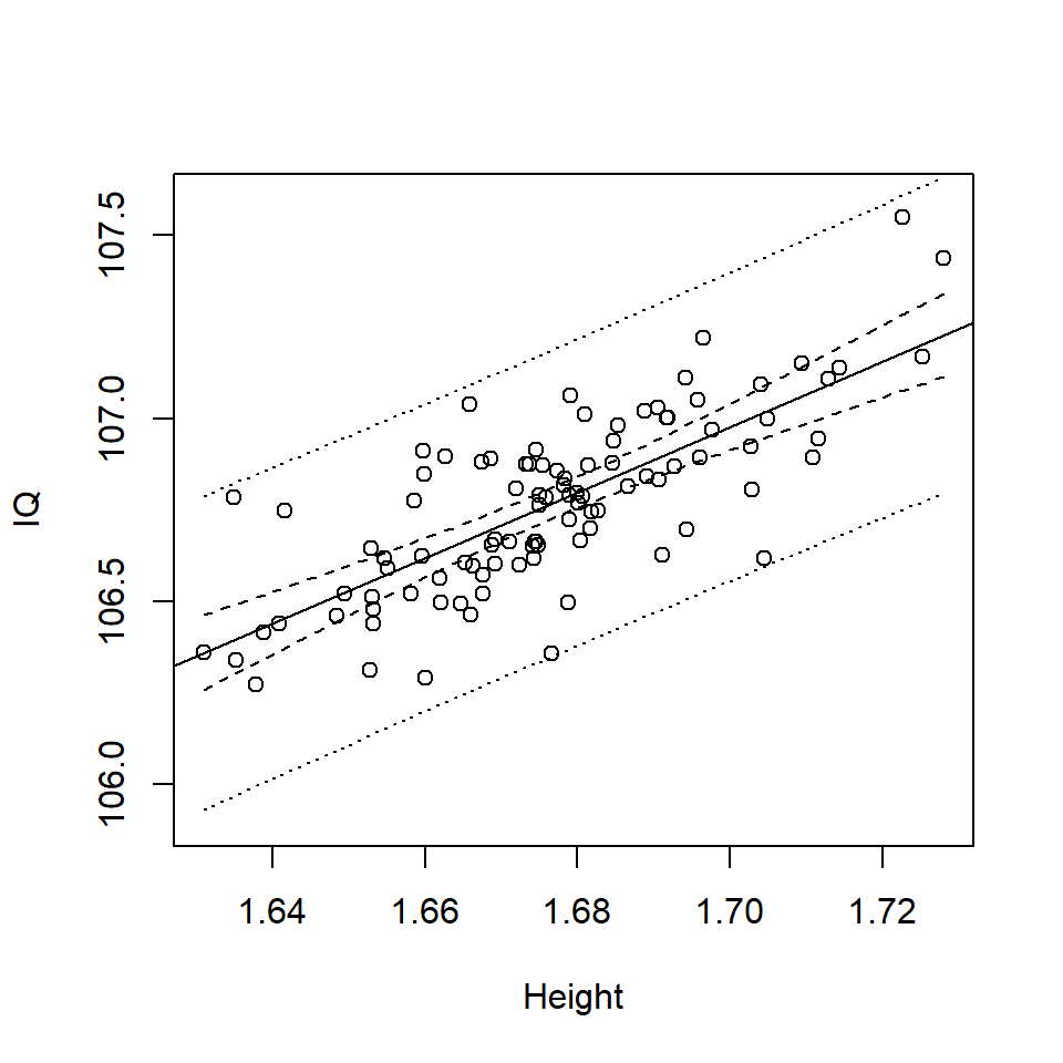
Figure 17.4: Scatterplot of Height (m) and IQ with confidence (dashes) and prediction intervals (dots) around the best fit line (solid line).
Notice that the prediction interval is much wider than the confidence interval (Figure 17.4):
- The confidence interval considers the uncertainty in the mean response, which essentially relates to the uncertainty in the estimated regression coefficients (i.e. \(\hat \beta\)’s).
- The prediction interval considers the uncertainty in the individual prediction which includes the uncertainty in the estimated regression coefficients (i.e. \(\hat \beta\)’s) plus the uncertainty in the prediction (i.e. the variance of the error).
Example An interesting application of regression, using a slightly more complicated regression technique that allowed curved fits is shown in Figure (Figure 17.5). Of interest was the relationship of jaw size to body length in giant squid. If we know this, undigested squid jaws found in sperm whales can be used to predict the size of squid sperm whales feed on. Here the uncertainty in the actual individual squid was of interest and so prediction intervals were calculated as well as a confidence interval. The prediction interval for body length of the longest jaw actually found in a sperm whale is given by the vertical green line. The longest mantle length measured is given by the horizontal green line. Statistics suggests some giant squid grow rather large!! Although this is based on an extrapolation (Paxton 2016).
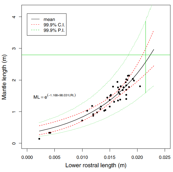
Figure 17.5: Regression of mantle length of lower rostral length in squid. The black line is the best fit line
17.4 Prediction in multiple regression
Prediction in multiple regression is carried out in the same way as in the simple regression case (although the calculation of the standard error is more complicated).
In R, a data frame with all the relevant covariates (i.e. those used in the model) must be created. To illustrate prediction for a multiple regression model, we return to a model fitted to the EIA data:
# Fit a linear model
linearAll <- lm(Density ~ XPos + YPos + DistCoast + Depth + as.factor(Month) + Phase,
                data=wfdata)
# Specify values for prediction
# Create dataframe
df.wf <- data.frame (XPos = mean (wfdata$XPos),
                     YPos = mean (wfdata$YPos),
                     DistCoast = 5,
                     Depth = 10,
                     Month = 4,
                     Phase = "C")
# Prediction
predict(linearAll, newdata=df.wf, se.fit=TRUE, interval="confidence",
        level=0.95)
$fit
fit lwr upr
1 3.568311 2.669927 4.466695
$se.fit
[1] 0.45835
$df
[1] 31492
$residual.scale
[1] 27.84424Hence, for the mean values of XPos and YPos, a DistCoast of 5km and Depth of 10m in Phase C in April, the predicted density of birds is 3.57 (95% 2.67-4.47) birds per km\(^2\).
It is possible to predict for any combinations of covariates even those that did not occur in the data. For example, the Depth and DistCoast values used in the above prediction may not actually occur together for any record in the observed data. This is a form of extrapolation and is dangerous (and potentially even pointless - why extrapolate from combinations of variables that do not occur in nature?).
Q17.1 For the following scenarios decide whether confidence intervals or prediction intervals would be more appropriate.
a. Estimation of the rate of change of population size of a new pest species entering an exploited environment.
b. Estimation of the heart rate in a clinical trial as a side effect of an experimental drug.
c. Estimation of the spatial density of an animal population.
d. Estimate of the relationship of IQ to height as part of a psychological investigation.
17.5 Summary
Given a fitted equation, obtaining a point estimate from a linear model is straightforward although care should be taken if extrapolation is being undertaken beyond the range of the data. Estimation of the uncertainty is more complex and requires decisions about \(\alpha\) and whether confidence or prediction intervals are required.
17.5.1 Learning objectives
At the end of this chapter you should be able to:
- predict from a given fitted model
- understand when to use confidence or prediction intervals.
17.6 Answers
Q17.1 Whether confidence intervals or prediction intervals are more appropriate is very contextual.
Q17.1 a. Here the emphasis is on the rate of change estimated by the gradient of a regression. So here a confidence interval on the gradient would be most appropriate.
Q17.1 b. In this case presumably safety is an issue so a plausible range of values for individuals is a primary concern so a prediction interval would be most appropriate.
Q17.1 c. If the interest was conservation then perhaps a prediction interval would be more appropriate, as that relates to the actual numbers of individuals. This is seldom done in practice however.
Q17.1 d. Here presumably the relationship is of more theoretical interest than practical policy so probably confidence intervals are relevant.