Chapter 10 Statistical Power
Nearly all men can stand adversity, but if you want to test a man’s character, give him power.
Misattributed to Abraham Lincoln.
10.1 Introduction
Statistical power is a measure of our ability to detect differences/effects given they actually do exist. In more formal statistical terms, it is our ability to reject the null hypothesis when it really should be rejected. Typically the question of power is raised in the planning of a study, e.g. ‘What should the sample size be in order to detect a given effect, if one is present?’ Alternatively, one could ask ‘What effect size could be detected, given a certain sample size?’
It is obvious when thinking about hypothesis tests that the probability of a result depends on both the underlying effect size and the sample size.
The idea of power is intimately connected to the Type II errors. Remember that a
- Type I error is the probability of incorrectly rejecting \(H_0\) i.e. a false positive
- Type II error is the probability of incorrectly failing to reject \(H_0\) i.e. a false negative.
These are shown in Table 10.1 along with the correct decisions. We control Type I errors in hypothesis tests by setting the threshold \(p\)-value (i.e. Type I error = \(\alpha\)) but so far we have not considered controlling Type II errors (\(\beta\)) in tests. In fact, the Type II error rate can be more difficult to calculate.
(#tab:type1and2) Type I and Type II errors
| Outcome of test | H\(_0\) True | H\(_0\) False |
|---|---|---|
| Reject H\(_0\) | Type I Error, \(\alpha\) | Correct decision |
| Fail to reject H\(_0\) | Correct decision | Type II Error, \(\beta\) |
Statistical power is given by (\(1-\beta\)) - this is the probability we correctly reject \(H_0\).
Q9.1 Given what you know of statistical power so far, what aspects of a statistical test do you think would increase power?
Calculating power requires we know (or speculate) about what the alternative hypothesis, \(H_1\), is - something we are usually very vague about. Similar to other hypothesis tests, our probability calculations are conditional on some hypothesised state being true.
10.2 A motivating example - Environmental impact assessment
Wind and tidal current turbines (Figure 10.1) are being built around the world to provide green energy. Typically, as part of the environmental impact associated with such construction, people consider the effects of the turbines on wildlife before being built, during development and when they are in operation. The impact may be an actual population change caused by the turbines or a redistribution of the population caused by the turbines.

Figure 10.1: A tidal current turbine.
Typically, the impacts are assessed by means of surveys of animals, for example, observers counting the animals present at various times and recording their locations and estimating the animal populations. However, the distribution and number of animals might be effected by a number of other variables, such as tide-state, time of day, season etc., as well as the turbines.
If no impact was found, this might be due to the fact that not enough surveying was undertaken. So a typical question might be, ‘If animal numbers decreased by half after turbine construction, what amount of survey effort would be required to detect that change?’ Alternatively, a range of scenarios might be considered, as in (Table ??), where different population effects are considered as well as two different sampling regimes (i.e. longer monitoring times).

Figure 10.2: Power (expressed as percentages) to detect an effect under different scenarios.
- For example, we would expect to detect a 20% reduction in the population if a further 6 months data are collected with a power of nearly 0.9.
Power calculations are often required in order to determine how much data to collect. This will depend on:
- How big an effect do you need/hope to detect?
- How much variability is in the system?
- What level of power is needed?
Armed with this information, we can advise on sample size, \(n\), to meet these specifications. Knowing the variability is the crucial issue; estimates might be obtainable from previous studies, a new pilot study or as a last resort, a guess. An estimate of variance from a pilot study might be inaccurate if sample size was low.
10.3 Calculating power
(Example modified from Larsen & Marx (2006))
Imagine there is a new fuel additive that is expected to increase the fuel efficiency for vehicles. The underlying fuel efficiency with the standard fuel is assumed to be 25 mpg. It is thought an improvement of at least 3% in fuel efficiency would be substantial enough for the additive to be taken to market. A trial is planned with the intention of detecting whether fuel efficiency with the additive has increased from 25 to 26 mpg (i.e. an approximate 3% increase) or even more.
We need to first identify our assumptions:
- Fuel efficiency in cars is normally distributed.
- The standard deviation of efficiency in cars is claimed to be \(\sigma\) = 2.4. We assume this is known (rather than estimated).
Assuming an effect size (improvement) to 26 mpg is desired, and a sample size of 30, what is the power and Type II error associated with this (one-sided) test scenario?
The underlying hypothesis test here is a one sample \(z\) test (because \(\sigma\) is known; if this were estimated, we would use a \(t\) test). The null and alternative hypotheses are:
\(H_0\): \(\hat \mu = 25\) \(H_1\): \(\hat \mu > 25\)
The test is one-tailed because we are considering an improvement in efficiency. It would be two-tailed is we were considering a difference in efficiency between the two fuels.
The test statistic is given by
\[ z_{stat} = \frac{\textrm{data-estimate} - \textrm{hypothesised value}}{\textrm{standard error(data-estimate)}} = \frac{\hat \mu - \textrm{hypothesised value}}{\frac{\sigma}{\sqrt{n}}}\] We would reject \(H_0\) if \(z_{stat}\) is greater than the critical value, \(z_{crit}\), i.e. \(z_{stat} > z_{crit}\):
\[ \frac{\hat \mu - \textrm{hypothesised value}}{\frac{\sigma}{\sqrt{n}}} > z_{crit}\] Thus, we can rearrange this expression to provide a value of \(\hat \mu\) that would be required to reject \(H_0\):
\[\hat \mu > \textrm{hypothesised value} + \frac{\sigma}{\sqrt{n}}z_{crit}\] Assuming the Type I error is 5%, (\(\alpha\) = 0.05), we know that the one-tailed critical value, \(z_{crit}\), is:
qnorm(p=0.95)[1] 1.644854The hypothesised value is 25, so that the critical value that would cause us to reject \(H_0\) can be calculated as follows:
\[25 + 1.644854 \times \frac{2.4}{\sqrt{30}} = 25.72\]
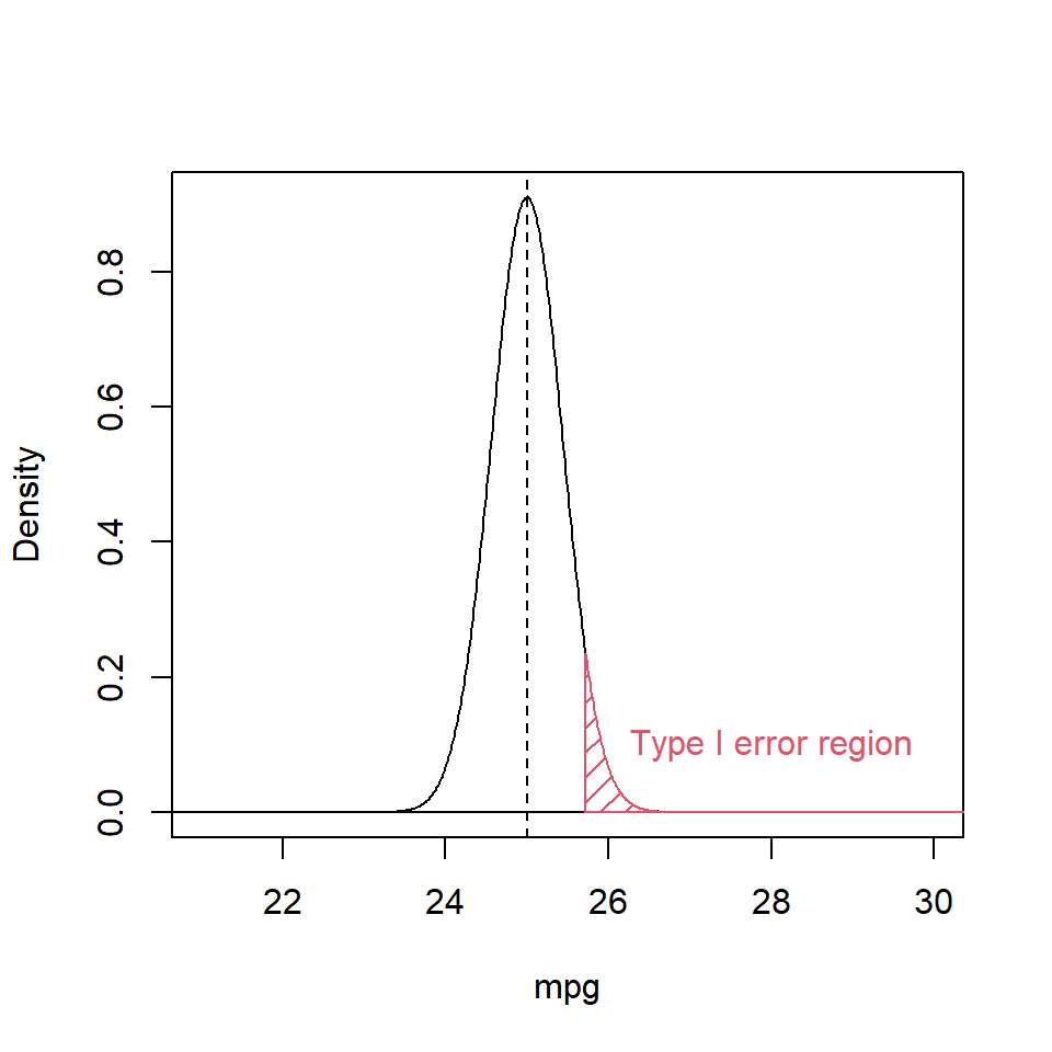
Figure 10.3 shows the probability density function under the null hypothesis i.e. \(N(\mu=25, \sigma=2.4)\). The red shaded area indicates critical value that would lead us to rejecting the null hypothesis under \(\alpha = 0.05\).

Figure 10.3: Probability density function of the reference distribution showing the Type I error region (shaded red).
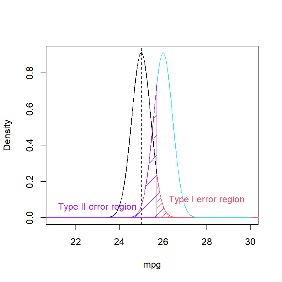
Hence, if our sample had a mean greater than 25.72 mpg we would reject \(H_0\). In rejecting the Null hypothesis we are at risk of making a Type I error. The Type II error, needs to be considered as well (Figure 10.4), relative to the alternative hypothesis. If \(H_1\) were true with its greater mean, and had the same standard deviation, we would produce false negatives (Type II errors) by falling left of this decision boundary.

Figure 10.4: Probability density function of reference distribution showing the Type I error region (shaded red) and the Type II error region (shaded purple).
To calculate the purple false negative area if \(\mu = 26\) in R:
pnorm(q=25.72, mean=26, sd=2.4/sqrt(30), lower.tail=TRUE)[1] 0.2614083- Thus, a Type II error occurs about 26.1% of the time.
- Power is \(1-\beta = 1 - 0.2614 = 0.7386\) i.e. 73.9% Therefore, we would fail to find evidence of a 1 mpg improvement almost a quarter the time.
10.3.1 Increasing the power
In the above case the power might be thought of as not very high. The obvious adaptions to make an improvements to this poor power are:
- Increasing precision through larger samples.
- Increasing precision through controlling variability (e.g. testing on a standardised track or the like).
- Accept a higher Type I error.
- Have a fuel additive that is expected to have improvements much greater than 1 mpg.
10.3.1.1 Increasing the sample size
What happens if \(n\) is doubled?
- The decision boundary is now at:
decisionBound <- 25+1.644854*2.4/sqrt(60)

decisionBound
[1] 25.50964Therefore the false negative rate is
pnorm(q=decisionBound, mean=26, sd=2.4/sqrt(60))[1] 0.05675267This means our Type II error is about 5.7% - a power of 94.3%. A power of 80% is frequently used as the goal when planning studies and experiments.
10.3.1.2 Increasing the effect size
Bigger changes in effect size would give higher power too, for example, we could consider 26.5 mpg instead of 26 mpg:
pnorm(q=decisionBound, mean=26.5, sd=2.4/sqrt(60))[1] 0.0006958301Power is now therefore 1 - 0.0007 = 99.9%; increasing the signal-to-noise ratio improves power.
10.3.1.3 Accepting a higher Type I error rate
Accepting an increased Type I error (e.g. \(\alpha=10\%\)) similarly improves power - it lowers the decision boundary in this problem, but this might be undesirable.
qnorm(p=0.9)[1] 1.281552decisionBound <- 25+qnorm(0.9)*2.4/sqrt(30)
decisionBound[1] 25.56155pnorm(q=decisionBound, mean=26, sd=2.4/sqrt(30))[1] 0.1585039Therefore the new power is 1 - 15.9 = 84.1%
- Given a Type II error of 26.1% versus 15.9% before (power moves from 73.9% originally to 84.1%).
Essentially, we are trading the probability of making one type of error for another.
10.3.2 Power by simulation
The above is a theoretical approach to the calculation of power; frequently these days, power is estimated by simulation. This is often a more intuitive approach.
Using the above case, we assume the true mean was normally distributed with mean 26 mpg and standard deviation 2.4. If 1000 samples (of size 30) are randomly generated from this distribution and the sample mean calculated each time, the proportion of the means greater than the critical value from the Null distribution (i.e. assuming \(\mu\) =25) would give the power. The code below implements this process.
# Initialise vector to store results
value <- NA
set.seed (101)
# Critical value
zcrit <- qnorm (p=0.95, mean=25, sd=2.4/sqrt(30))

# Begin loop
for (i in 1:1000) {
  # Generate random sample
  samplepower <- rnorm (n=30, mean=26, sd=2.4) ###this is truth
  # Test mean of sample, if > zcrit value=1, otherwise value=0
  if (mean(samplepower) > zcrit) {value[i]=1}
  else {(value[i]=0)}
} # End loop

# Calculate proportion
power <- sum(value)/1000
power
[1] 0.757The generated power is similar to 73.8%, the value obtained above using a theoretical approach. If the number of iterations is increased the generated power converges ever closer to 73.8%.
Similarly, if the sample size is increased to 60 (i.e. n = 60 above) then an answer similar to the theoretical figure of approximately 94.3% is obtained.
# Initialise vector to store results
value <- NA
set.seed (101)
# Critical value
zcrit <- qnorm (p=0.95, mean=25, sd=2.4/sqrt(60))

# Begin loop
for (i in 1:1000) {
  # Generate random sample
  samplepower <- rnorm (n=60, mean=26, sd=2.4) ###this is truth
  # Test mean of sample, if > zcrit value=1, otherwise value=0
  if (mean(samplepower) > zcrit) {value[i]=1}
  else {(value[i]=0)}
} # End loop

# Calculate proportion
power <- sum(value)/1000
power
[1] 0.95An interactive example of simulation based power analysis with varying sample size is in Figure 10.5. There is also a live version here
Figure 10.5: An example of simulation based power analysis. You can see a live version by clicking here
10.3.3 Multiple comparisons
As discussed previously, when we make multiple comparisons and we adjust the family wise error rate (see the previous chapter) we are decreasing the risk of a Type I error but increasing the risk of a Type II error leading to a lower power.
- We make our Type I error boundaries more stringent (broader) i.e. lower threshold \(p\)-values.
- We are trading errors at some level, i.e., if the Type II errors increase, the power decreases.
10.4 Summary
Power should be an essential component of planning a statistical investigation. As mentioned above, a common convention is that a study should have power of c. 80% to be viable. Small sample sizes, trying to distinguish very small effect sizes and sloppy measurement with high variance will decrease the power of a test and lead to a low probability of rejecting \(H_0\). If these activities are undertaken to deliberately fail to reject \(H_0\) then this would be scientific misconduct.
There are myths propagated in some scientific disciplines about statistical power, namely that the power of a test can be assessed post-hoc to determine if the found negative results are justified. To be blunt, this is nonsense. Power is numerically related to probability for a given null hypothesis, therefore, any result which fails to reject the null hypothesis will have low power. It is meaningless to calculate power post-hoc as a way of ascertaining the appropriateness of a null result.
10.4.1 Learning Objectives
At the end of this chapter you should:
- understand power and its appropriate uses
- calculate simple power statistics, and
- understand when power should not be used.
10.5 Answers
Q9.1 Power is all about the signal to noise ratio, therefore, we can either:
- increase the signal i.e. assume a bigger effect size or
- decrease the noise i.e. increase the precision typically by increasing sample size.