Chapter 19 The Next Steps
19.1 Introduction
It cannot be stressed enough that if the assumptions of a statistical model, or indeed a statistical test, are not met, then any conclusions drawn from that model/test may be erroneous. This is the case for both the simple and more complex models presented in this module. If the assumptions are not met there may be adjustments, alternative tests or more advanced statistical methods that can be implemented. Here; we explore some simple ways to overcome such problems with distributional assumptions as well as introduce some advanced methods that may be available.
19.2 Solving the assumptional problems
Previous chapters have described model diagnostics to check the model assumptions, and so, armed with this information, we can revisit, our conclusions about what influences density in the EIA data set for example, and evaluate the model in terms of the assumptions. However, what happens if assumptions (for any linear model) are not met? While this is a cause for concern, there are various approaches that can be adopted in these circumstances.
19.2.1 Example: The EIA data
At this point it appears from previous chapters there are no differences in the average density across the three development phases but some evidence for differences in the easting (X-coordinate) relationship across phases.
While this may be indicative of the true situation, in practise we need to do more to be able to answer our research questions. Although our model appears to fit the data adequately (\(R^2\)-wise), our model returns impossible predictions (negative density estimates) and the assumptions appear to be violated. More specifically the problems are:
- The model for signal is likely a little simple:
- The variables
XandYare spatial co-ordinates and using simple lines to describe them may not be adequate to capture all the pattern in density.
- The variables
- The model for noise is wrong:
- The residuals are not normal in shape (with the implied constant variance).
- The estimated errors don’t appear independent (not surprisingly because density was measured at locations along lines and density at locations which are close together may be similar).
Therefore, the conclusions from the model are unsafe and cannot be relied upon. This is a very common situation in practise.
What can be done?
19.2.2 Oddly distributed residuals
One important assumption of the linear models discussed so far is that the residuals are normally distributed with the same variance i.e. \(\epsilon_i \sim N(0, \sigma^2)\); this assumption is not always met in practise. If the residuals are not normally distributed, then various options are available to account for this: the dependent data (response) can be transformed (e.g. by taking the logarithm or square root) to address the distributional shape problems. This is effective but the consequence is that:
the geometric mean is modelled rather than the arithmetic mean if for example a log transformation is used,
interactions found in the untransformed data may disappear (this may not be a problem, a multiplicative relationship has just become a additive one).
Generalised linear models (GLMs) allow different shaped distributions for noise. These models are covered in another course.
Generalised Least Squares (GLS) methods can help with non-constant variance. These methods are also covered in another module.
A bootstrap can be used to obtain approximate measures of uncertainty that do not rely on the distributional assumptions (see below).
19.2.3 Non-independence
We have four options if the data are not independent. We can:
- ignore the correlation in the residuals (easy but unwise).
- investigate other key variables that can account for the dependence.
- try to remove the correlation in model residuals by sub-setting the data (for example, re-run analysis using every 20th observation; this reduces the sample size and wastes information)
- account for the correlation using, for example, a Generalized Least Squares (GLS) or Generalized Estimating Equation (GEE) model - this is another course.
19.2.4 Non-linearity
If a straight line is not appropriate then we can use:
- more complex linear models (i.e. more variables),
- non-linear (in the everyday sense) functions (i.e. Generalised Additive Models GAMs) or
- many other predictive modelling tools, if you only care about prediction (rather than explanation/description) of the response.
19.2.5 Bootstrapping
The bootstrap has been described previously. You can think of it as simulating more samples, but using our data as a basis for determining uncertainty. In general, the bootstrap procedure consists of:
- generating a new data set of the same dimensions, by sampling the rows of our original data with replacement (a non-parametric bootstrap),
- we do this many times and fit models each time, storing the estimates of the statistic of interest.
- This shows roughly how much things might change if we were to have another sample.
- The collective set of estimates provides a distribution of estimates, from which we infer/generate confidence intervals for the parameters.
Here we implement an example of bootstrapping a simple linear regression model to obtain an approximate confidence interval for the regression coefficients (i.e. the intercept and slope). Suppose that we have fitted a simple linear regression model and we are reasonably happy that a simple linear model is appropriate (i.e. the model for the signal is suitable) and the independence assumption is valid. However, diagnostic plots indicate that the residuals are not normally distributed. We would like to interpret the parameter estimates - in particular with consideration to the uncertainty (e.g. confidence intervals) and the conventional CI may be incorrect if the distributional assumptions are violated.
As indicated, the general bootstrap procedure is:
- Sample the data, with replacement, to give an equivalently dimensioned data set
- Fit the linear model to this new ‘bootstrap’ sample - store the parameter estimates
- Repeat this process many times (e.g. at least 1000 times)
- Take, say, the central 95% of these estimates as an approximate 95% confidence interval
The advantage of a bootstrap is that if the residual distribution is very skewed, then you’ll naturally get skewed 95% CIs which are more appropriate.
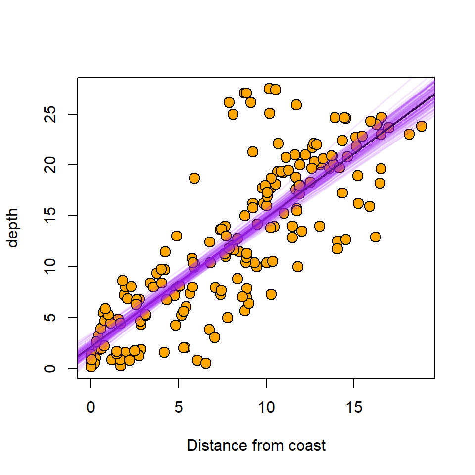
Example In the code below a simple linear regression model is fitted to the EIA data with Depth as the response and DistCoast as the explanatory variable. A bootstrap procedure is then implemented to obtain CI for the regression coefficients. For ease of producing the plots, the process was repeated only a 100 times, but properly it should be at least 1000.
library(dplyr)

# Create an object to store results
bootCoefs<- array(dim = c(100, 2))

# Select only necessary columns
workingDataorig <- wfdata %>% select(DistCoast, Depth)

# Fit model to original data
model1 <- lm (Depth ~ DistCoast, data=workingDataorig)

# Start bootstrap loop
for (i in 1:100) {
  # Select a random subset (to make computations tractable for example)
  workingData <- workingDataorig[sample(1:nrow(workingDataorig), 200),]
  # Generate bootstrap sample of row numbers
  bootIndex <- sample(1:nrow(workingData), nrow(workingData), replace=T)
  # Select data based on sample of row numbers
  bootData <- workingData[bootIndex, ]
  # Fit linear model
  bootLM <- lm(Depth ~ DistCoast, data=bootData)
  # Store coefficients
  bootCoefs[i,] <- coefficients(bootLM)
}
# Obtain 95% quantiles for the coefficients
bootCI <- apply(bootCoefs, 2, quantile, probs = c(0.025, 0.975))
# Add column names
colnames(bootCI) <- c('Intercept', 'Slope')

# Use these to define a colour with some transparancy (alpha)
myCol <- rgb(160, 32, 240, alpha=30, max=255)

# Plot data and all bootstrap regression lines
plot(workingData$DistCoast, workingData$Depth, cex=1.5, xlab='Distance from coast',
       ylab="depth", bg='orange', pch = 21,
       main='', sub='')
# Original regression line (black)
abline (model1, lwd=2)
# Add bootstrap regression lines
apply(bootCoefs, 1, abline, col=myCol, lwd=1.5)
Figure 19.1: The best fit line (black) with bootstrap replicate best fit lines (purple).
NULLFrom the bootstrap we can get approximate 95% CIs from the central 95% of parameter estimates.Not that the CIs obtained here are for the parameters NOT for the predictions (see Chapter 17 for that).
bootCI Intercept Slope
2.5% 1.067695 1.151715
97.5% 3.308414 1.375905The conventional 95% CI (i.e. based on the distributional assumptions of the linear model) are:
# Fit a simple linear model
model1 <- lm(Depth ~ DistCoast, data=workingData)
t(confint(model1))
(Intercept) DistCoast
2.5 % 0.6012957 1.187548
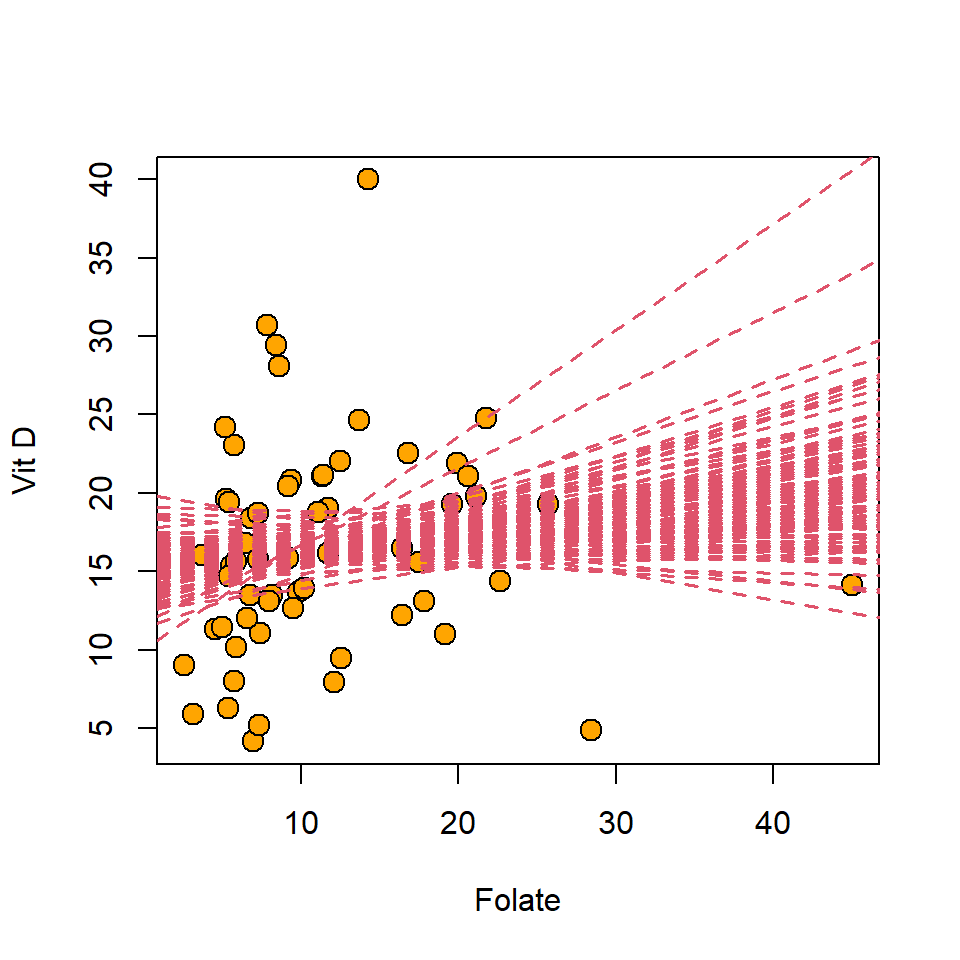
97.5 % 2.8930065 1.432019Example The bootstrap procedure is applied to the medical data set where vitamin D level is the response and folate is used as an explanatory variable in a simple linear regression model.
# Fit simple linear regression model to all the data
modelfolate <- lm(vitdresul ~ folate, data=meddata)

# Create object to store results
bootCoefs <- array(dim = c(100, 2))

# Bootstrap loop
for (i in 1:100) {
  # Generate sample of rows
  bootIndex <- sample(1:nrow(meddata), nrow(meddata), replace=T)
  # Select data based on sample
  bootData <- meddata[bootIndex, ]
  # Fit linear model
  bootLM<- lm(vitdresul ~ folate, data=bootData)
  # Save regression coefficients
  bootCoefs[i,] <- coefficients(bootLM)
}
# Obtain 95% quantiles
bootCI<- apply(bootCoefs, 2, quantile, probs = c(0.025, 0.975))
# Add names
colnames(bootCI) <- c('Intercept', 'Slope')
# Print results
bootCI
Intercept Slope
2.5% 11.98095 -0.05500593
97.5% 18.66542 0.35425516The bootstrapped regression lines are shown in Figure 19.2.

Figure 19.2: Bootstrap replicate best fit lines for an analysis of the medical data set.
NULLThere is much that could be said about the bootstrap, but this goes beyond this course. Suffice it to say it can be incredibly useful see Davison & Hinckley (1997).
19.3 Summary
Diagnostic plots indicate whether the assumptions of the linear model are valid. If not, there are several solutions to violated linear model assumptions.
Non-normality can be tackled by bootstrapping, transformations, or alternative models beyond the level of this course
Non-independence is a real problem - need alternative methods beyond this course.
More complex or better models for the signal - alternative models beyond this course.
Beyond the linear model
As already hinted, linear models are part of a far wider class of models that can handle complex data in a regression framework.
As well as the model assumptions to check, there are other considerations to take account of. For example are your samples representative of the population under consideration i.e. does the result have external validity? Is the (experimental) design of data collection such that no biases could occur. This is far more difficult to ensure than might be thought. Aspects such as how statistical data should be presented in order to provide useful summaries? What is best practise? All this and more is considered in the module Statistical Thinking.
19.3.1 Learning outcomes
At this end of this chapter you should be able to:
- use some methods to overcome assumption violations of the linear model, and
- recognise when methods beyond this course may be appropriate.