Chapter 16 Interactions and the Linear Model
To bring this back to a non-metaphorical level, I am suggesting that Black women can experience discrimination in ways that are both similar to and different from those experienced by
white women and Black men. Black women sometimes experience discrimination in ways similar to white women’s experiences; sometimes they share very similar experiences with Black men. Yet
often they experience double-discrimination-the combined effects of practices which discriminate on the basis of race, and on the basis of sex. And sometimes, they experience discrimination as
Black women-not the sum of race and sex discrimination, but as Black women.
Kimberlé Crenshaw (1989)
16.1 Introduction
So far, we have only considered linear models that include main effects; so in the following model,
\[y = \beta_0 + \beta_1x_1 + \beta_2 x_2 + \epsilon\] where
- \(y\) is the response,
- \(x_1\) and \(x_2\) are continuous variable main effects;
- \(\beta_0\) is the intercept,
- \(\beta_1\) and \(\beta_2\) are the gradients associated with \(x_1\) and \(x_2\), respectively, and
- \(\epsilon\) is the error.
Alternatively, we might have a categorical and continuous variable as main effects: \[y = \beta_0 + \beta_{1_j} + \beta_2 x_2 + \epsilon\] where
- \(\beta_{1j}\) represents the intercept associated with a categorical variable level \(j\) (note, \(\beta_{1_1}=0\) if level 1 is used as a baseline/reference level).
However, we might also be interested in including interactions between variables.
One question that might be asked of the environmental impact assessment (EIA) data, for example, is whether there is any evidence for a spatial re-distribution of bird density across construction phases (A,B or C) of the wind farm. We can do this by asking if a particular sort of density pattern in the X or Y spatial direction differs across phases, i.e. does the effect on density of X or Y differ between the levels of phase. We call this sort of effect an interaction.
- Interaction is equivalent to the idea of “synergy” in chemistry or “intersectionality” in the humanities, or social sciences (see the quote by Kimberlé Crenshaw at the beginning of the chapter).
Example Say Drug A raised heartbeat by say 10 beats a minute and Drug B raises heartbeat by 20 beats per minute. Taken together they do not increase heartbeat by 30 beats per minute but reduce it by 10. There is a non-additive effect.
But what does an interaction mean in statistical terms? In this chapter we illustrate statistical interaction and how to include them in linear models.
16.1.1 Fitting different models
Let’s investigate human height as a function of leg length.
The data contains measurements for 100 males and 100 females, where the two groups differ in height (Figure 16.1). We see that height differs by sex, but how is that affected by leg length?
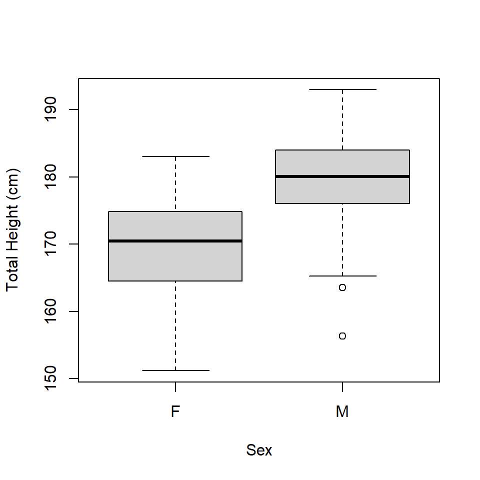
Figure 16.1: Boxplot of height by sex.
Exploratory analysis suggests that whilst females are generally shorter, the relationship between leg length and total height is the same in both sexes (Figure 16.2). There is a difference in the intercept but not in the gradient (slope) between the two sexes.
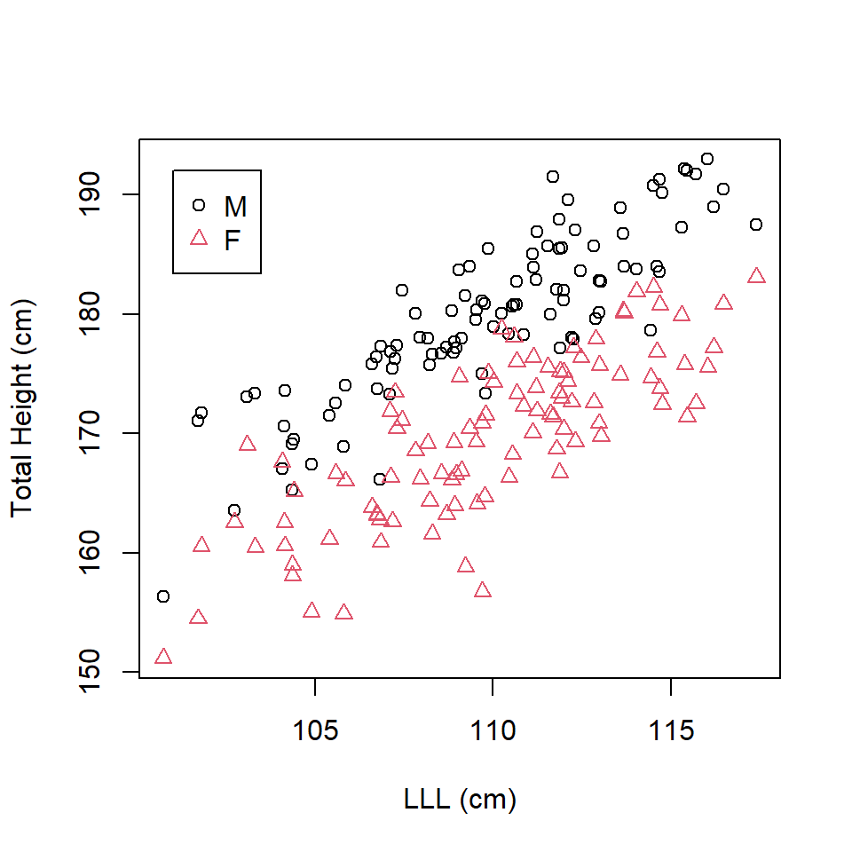
Figure 16.2: Scatterplot of left leg length and total height by sex.
This is confirmed by the regression analysis.
# Fit model
model_height1 <- lm(TotalHeight ~ Sex + LLL, data=heightdata)
# ANOVA
anova(model_height1)
Analysis of Variance Table
Response: TotalHeight
Df Sum Sq Mean Sq F value Pr(>F)
Sex 1 5110.8 5110.8 341.36 < 2.2e-16 ***
LLL 1 6646.5 6646.5 443.93 < 2.2e-16 ***
Residuals 197 2949.5 15.0
---
Signif. codes: 0 '***' 0.001 '**' 0.01 '*' 0.05 '.' 0.1 ' ' 1# Summary
summary (model_height1)
Call:
lm(formula = TotalHeight ~ Sex + LLL, data = heightdata)

Residuals:
     Min       1Q   Median       3Q      Max
-12.6939  -2.3477  -0.1715   2.6812   9.8925

Coefficients:
            Estimate Std. Error t value Pr(>|t|)
(Intercept)  -0.6919     8.0941  -0.085    0.932
SexM         10.1102     0.5472  18.476   <2e-16 ***
LLL           1.5507     0.0736  21.070   <2e-16 ***
---
Signif. codes:  0 '***' 0.001 '**' 0.01 '*' 0.05 '.' 0.1 ' ' 1

Residual standard error: 3.869 on 197 degrees of freedom
Multiple R-squared:  0.7994,    Adjusted R-squared:  0.7974
F-statistic: 392.6 on 2 and 197 DF,  p-value: < 2.2e-16
We can now obtain the best fit lines. The general model is:
\[\mathrm{TotalHeight} = \beta_0 + \beta_1\mathrm{Sex} + \beta_2\mathrm{LLL} + \epsilon\] The best fit line for females (baseline) is: \[\mathrm{\widehat{TotalHeight}_{Females}} = -0.6919 + 1.5507 \times \mathrm{LLL}\]
The best fit line for males is: \[\begin{align} \mathrm{\widehat{TotalHeight}_{Males}}& = -0.6919+ 10.1102 + 1.5507 \times \mathrm{LLL}\\ & = 9.4183 + 1.5507 \times \mathrm{LLL}\\ \end{align}\]
These lines can then be added to the scatter plots using the abline command where we supply the intercept (a=) and gradient (b=) (Figure 16.3).
# Create new variable for plotting colours/symbols
heightdata$SexNumeric <- ifelse(test=heightdata$Sex=="M", yes=1, no=2)

plot (heightdata$LLL, heightdata$TotalHeight, col=heightdata$SexNumeric,
      pch=heightdata$SexNumeric, xlab="LLL (cm)", ylab= "Total Height (cm)")
# Add legend
legend(101, 192, legend=c("M","F"), col=1:2, pch=1:2)
# Red dashes for females
abline (a=-0.6919, b=1.5507, col=2, lty=2)
# Black line for males
abline (a=(-0.6919 + 10.1102), b=1.5507)
Figure 16.3: Scatterplot of left leg length and total height by sex with best fit lines with different intercept terms.
Has this achieved what we want? We have not really allowed the model to consider the possibility that the relationship between LLL and total height differs between the sexes. We look at this now.
16.2 Fitting interaction terms
To test whether the relationship is different between the sexes we could fit regression lines to each sex independently and then examine the gradient terms in each model. However, this would halve our sample size in each case. An alternative is to allow the sex of the measured human to influence both intercept and the gradient of the best fit lines. Using Sex as a main effect allows for a different intercept (we have done this already). For an additional influence on gradient we need to specify an interaction term. We can do this in R by using the term : in the model formula between the variables of interest e.g.
# Fit model with interaction
model_height_interaction <- lm(TotalHeight ~ LLL + Sex + LLL:Sex,
                               data=heightdata)
summary(model_height_interaction)
Call:
lm(formula = TotalHeight ~ LLL + Sex + LLL:Sex, data = heightdata)

Residuals:
     Min       1Q   Median       3Q      Max
-12.7063  -2.4203  -0.0151   2.6133   9.3352

Coefficients:
            Estimate Std. Error t value Pr(>|t|)
(Intercept)   8.3556    11.4328   0.731    0.466
LLL           1.4683     0.1040  14.116   <2e-16 ***
SexM         -7.9850    16.1685  -0.494    0.622
LLL:SexM      0.1647     0.1471   1.120    0.264
---
Signif. codes:  0 '***' 0.001 '**' 0.01 '*' 0.05 '.' 0.1 ' ' 1

Residual standard error: 3.867 on 196 degrees of freedom
Multiple R-squared:  0.8007,    Adjusted R-squared:  0.7977
F-statistic: 262.5 on 3 and 196 DF,  p-value: < 2.2e-16
Here the coefficient of the interaction term acts as a modifier of the gradient coefficient for the non-baseline sex (Figure 16.4). The fitted equations for each sex are given below.
The best fit line for females (the baseline) is \[\mathrm{\widehat{TotalHeight}_{Females}} = 8.3556 + 1.4683 \times \mathrm{LLL}\] The best fit line for males is \[\begin{align} \mathrm{\widehat{TotalHeight}_{Males}} &= (8.3556 -7.9850) + (1.4683+0.1647) \times \mathrm{LLL}\\ & = 0.3706 + 1.633 \times \mathrm{LLL}\\ \end{align}\]
plot (heightdata$LLL, heightdata$TotalHeight, col=heightdata$SexNumeric,
      pch=heightdata$SexNumeric, xlab="LLL (cm)", ylab= "Total Height (cm)")
legend(101, 192, legend=c("M","F"), col=1:2, pch=1:2)
# Red dashes for females
abline (a=8.3556, b=1.4683, col=2, lty=2)
# Black line for males
abline (a=0.3706, b=1.633)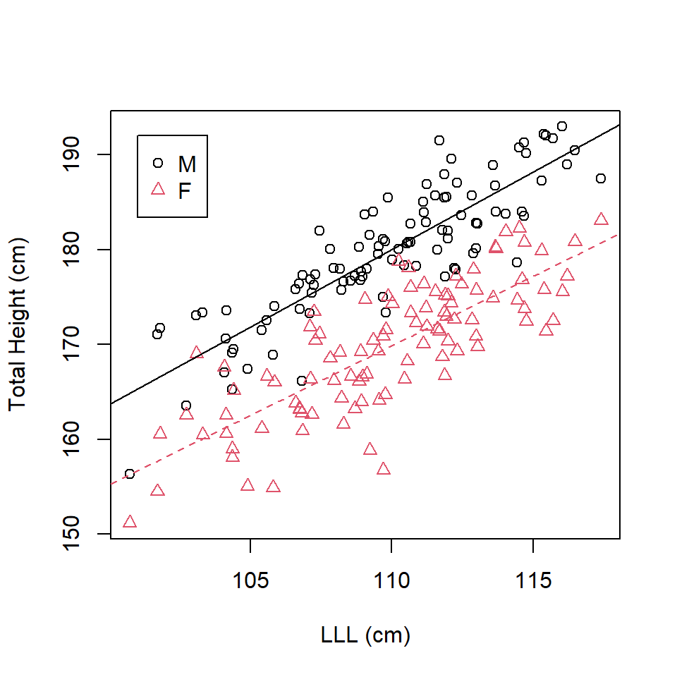
Figure 16.4: Scatterplot of left leg length and total height by sex with best fit lines from an interaction.
Even allowing for a change in gradient, the best fit lines are not too dissimilar and an anova table reveals no significant interaction effect (this could also be inferred from the summary table).
anova(model_height_interaction)Analysis of Variance Table
Response: TotalHeight
Df Sum Sq Mean Sq F value Pr(>F)
LLL 1 6646.5 6646.5 444.506 <2e-16 ***
Sex 1 5110.8 5110.8 341.798 <2e-16 ***
LLL:Sex 1 18.7 18.7 1.254 0.2642
Residuals 196 2930.7 15.0
---
Signif. codes: 0 '***' 0.001 '**' 0.01 '*' 0.05 '.' 0.1 ' ' 1However, here is a very different sample of some rather tall male and female humans (perhaps they are Dutch!) (Figure 16.5).
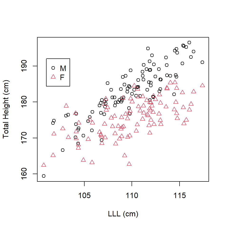
Figure 16.5: Scatterplot of total height in leg length in tall humans.
The relationship between LLL and TotalHeight is clearly different for each sex. This is confirmed by the summary output where the interaction term is significant.
model_height_interaction2 <- lm(TotalHeight ~ LLL + Sex + LLL:Sex, data=heightdata2)
anova (model_height_interaction2)
Analysis of Variance Table
Response: TotalHeight
Df Sum Sq Mean Sq F value Pr(>F)
LLL 1 4484.6 4484.6 300.171 < 2.2e-16 ***
Sex 1 2859.2 2859.2 191.375 < 2.2e-16 ***
LLL:Sex 1 419.6 419.6 28.082 3.114e-07 ***
Residuals 196 2928.3 14.9
---
Signif. codes: 0 '***' 0.001 '**' 0.01 '*' 0.05 '.' 0.1 ' ' 1summary (model_height_interaction2)
Call:
lm(formula = TotalHeight ~ LLL + Sex + LLL:Sex, data = heightdata2)

Residuals:
     Min       1Q   Median       3Q      Max
-12.6799  -2.4192  -0.0154   2.6185   9.3240

Coefficients:
            Estimate Std. Error t value Pr(>|t|)
(Intercept)  78.4027    11.4281   6.860 8.77e-11 ***
LLL           0.8842     0.1040   8.504 4.66e-15 ***
SexM        -78.0345    16.1618  -4.828 2.77e-06 ***
LLL:SexM      0.7792     0.1470   5.299 3.11e-07 ***
---
Signif. codes:  0 '***' 0.001 '**' 0.01 '*' 0.05 '.' 0.1 ' ' 1

Residual standard error: 3.865 on 196 degrees of freedom
Multiple R-squared:  0.7261,    Adjusted R-squared:  0.7219
F-statistic: 173.2 on 3 and 196 DF,  p-value: < 2.2e-16
The best fit lines are now:
For females (as females are the baseline): \[\mathrm{\widehat{TotalHeight}_{Females}} = 78.4027 + 0.8842 \times \mathrm{LLL}\] For males: \[\begin{align} \mathrm{\widehat{TotalHeight}_{Males}} & = (78.4027-78.0345) + (0.8842+0.7792) \times \mathrm{LLL}\\ & = 0.3682 + 1.6634 \times \mathrm{LLL}\\ \end{align}\]
which can then be plotted (Figure 16.6).
plot (heightdata2$LLL, heightdata2$TotalHeight, col=heightdata2$SexNumeric,
      pch=heightdata2$SexNumeric, xlab="LLL (cm)", ylab= "Total Height (cm)")
legend(101, 192, legend=c("M","F"), col=1:2, pch=1:2)
# Red dashes for females
abline(a=78.4027, b=0.8842, col=2, lty=2)
# Black line for males
abline(a=0.3682, b=1.6634)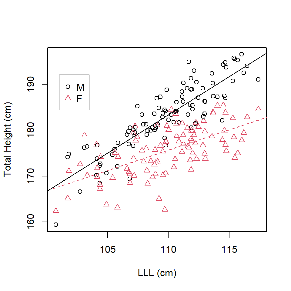
Figure 16.6: Scatterplot of total height on left leg length in tall humans.
Two things to note:
the intercepts are NOT the same for each sex because the \(y\) axis is not at \(x = 0\).
we have considered an interaction of a categorical variable with a continuous variable (= effect on the gradient).
16.2.1 Specifying interactions in model formulae
If we were to write the above model as a general equation it would be:
\[\mathrm{TotalHeight} = \beta_0 + \beta_{\textrm{Sex}_j} + \beta_2\mathrm{LLL} + \gamma_{\textrm{Sex}_j}\mathrm{LLL} + \epsilon \] or \[\mathrm{TotalHeight} = \beta_0 + \beta_{\textrm{Sex}_j} + (\beta_2 + \gamma_{\textrm{Sex}_j})\mathrm{LLL} + \epsilon \]
where
\(\beta_0\) is the intercept,
\(\beta_{\textrm{Sex}_j}\) is the intercept coefficient associated with Sex category \(j\) (i.e. Male or Female),
\(\beta_2\) is the gradient coefficient associated with \(LLL\),
\(\gamma_{\textrm{Sex}_j}\) is the gradient coefficient associated with Sex category \(j\) for \(LLL\), and
\(\epsilon\) is the error term.
In this example, \(\beta_{\textrm{Sex}_\textrm{Female}}=0\) and \(\gamma_{\textrm{Sex}_\textrm{Female}}=0\) because ‘Female’ is the baseline or reference level.
Writing this type of equation in even more general notation (e.g. with \(y\) and \(x\)), then we have:
\[y = \beta_0 + \beta_{1_j} + \beta_2 x_2 + \gamma_{1_j}x_2 + \epsilon\] \[y = \beta_0 + \beta_{1_j} + (\beta_2 + \gamma_{1_j})x_2 + \epsilon\]
where
\(\beta_0\) is the intercept,
\(\beta_{1j}\) in the intercept coefficient associated with categorical variable 1 level \(j\),
\(\beta_2\) is gradient associated with continuous variable \(x_2\),
\(\gamma_{1j}\) is the gradient associated with categorical variable 1 level \(j\) and \(x_2\), and
\(\epsilon\) is the error term.
An interaction of a continuous variable with another continuous variable would affect the gradient too, but in 3 dimensions (i.e. that interaction would have to be visualized using 3D plots or similar, e.g. section 3.6.4 and 3.6.5).
Algebraically, an interaction between two continuous variables (\(x_1\) and \(x_2\)) is (simply) given as:
\[y = \beta_0 + \beta_1 x_1 + \beta_2 x_2 + \beta_3 x_1x_2 + \epsilon\]
An interaction of two categorical variables would affect the intercepts and be illustrated (assuming no other variables) by a 3D bar chart or similar.
Algebraically, an interaction between two categorical variables (denoted by \(1\) and \(2\)) is given as:
\[y = \beta_0 + \beta_{1_j} + \beta_{2_k} + \gamma_{12_{jk}} + \epsilon\] where
\(\beta_1\) and \(\beta_2\) are the intercepts associated with categorical variables \(1\) and \(2\), level \(j\) and \(k\), respectively.
\(\gamma_{12_{jk}}\) is the intercept associated with the interaction between categorical variables 1 and 2, level \(j\) and \(k\).
We can actually also have interactions of 3, or more, variables but the interpretation of such models can be very difficult and the data need to be well supported (i.e. you need cases of all the different combinations of the variable levels in the factorial case).
16.3 Interactions in practise
In this section, we return to two data sets that we have introduced in previous chapters and look at including interactions.
Example We can implement an interaction(s) in our model to explain density by including phase:X and phase:Y terms:
Call:
lm(formula = Density ~ XPos + YPos + DistCoast + Depth + as.factor(Month) +
    Phase + XPos:Phase + YPos:Phase, data = wfdata)

Residuals:
    Min      1Q  Median      3Q     Max
 -12.27   -5.28   -2.96   -0.16 1715.13

Coefficients:
                    Estimate Std. Error t value Pr(>|t|)
(Intercept)       3279.23859  330.78931   9.913  < 2e-16 ***
XPos                 0.08446    0.01958   4.314 1.61e-05 ***
YPos                -0.55007    0.05445 -10.102  < 2e-16 ***
DistCoast           -0.31486    0.06937  -4.539 5.68e-06 ***
Depth               -0.45478    0.04077 -11.154  < 2e-16 ***
as.factor(Month)2    0.52526    0.53628   0.979  0.32737
as.factor(Month)3    3.15320    0.46242   6.819 9.34e-12 ***
as.factor(Month)4    0.65421    0.45868   1.426  0.15379
PhaseB             104.08871  325.32389   0.320  0.74901
PhaseC            -223.71597  404.53413  -0.553  0.58025
XPos:PhaseB          0.07107    0.02572   2.764  0.00572 **
XPos:PhaseC          0.00631    0.03135   0.201  0.84048
YPos:PhaseB         -0.02525    0.05329  -0.474  0.63564
YPos:PhaseC          0.03603    0.06646   0.542  0.58770
---
Signif. codes:  0 ‘***’ 0.001 ‘**’ 0.01 ‘*’ 0.05 ‘.’ 0.1 ‘ ’ 1

Residual standard error: 27.84 on 31488 degrees of freedom
Multiple R-squared:  0.01512,   Adjusted R-squared:  0.01472
F-statistic: 37.19 on 13 and 31488 DF,  p-value: < 2.2e-16
There are rules for including interaction terms in a model:
(Unless you are an advanced user) if you have an interaction term you should also include the main effects terms associated with the interaction. In the example above, the model includes
Phase,XPosandYPosas main effects.If the interaction is significant, the \(p\)-values associated with the main effects are irrelevant and so the main effects are retained.
If \(p\)-value selection is in operation and the interaction is removed, the main effects should not be removed before re-evaluating the model.
Interactions always come last in the sequence of predictors.
A phase-based interaction term
In our new interaction-based model (above) we have:
\[\begin{equation} y_{it}=\beta_{0}+\beta_1x_{1i}+\beta_2x_{2i}+\beta_3x_{3i}+...+\beta_{13}x_{13i} \end{equation}\]
where \(\beta_{1}-\beta_9\) and \(x_{1i}-x_{9i}\) are as described before and relate to XPos, YPos, DistCoast, Depth, Month and Phase. The new aspects of the output are as follows:
XPos:phaseB: \(\beta_{10}\) is the expected change in the slope coefficient for the XPos relationship in phase B compared with the XPos relationship in phase AXPos:phaseC: \(\beta_{11}\) is the expected change in the slope coefficient for the XPos relationship in phase C compared with the XPos relationship in phase AYPos:phaseB: \(\beta_{12}\) is the expected change in the slope coefficient for the YPos relationship in phase B compared with the YPos relationship in phase AYPos:phaseC: \(\beta_{13}\) is the expected change in the slope coefficient for the YPos relationship in phase C compared with the YPos relationship in phase A
The uncertainty associated with the interaction-based estimates result in:
- no statistically significant difference between the
XPos-slope coefficient for phase A compared with phase C (XPos:phaseC; \(p\)-value=0.840)
- no statistically significant difference between the
YPos-slope coefficient for phase B compared with phase A (YPos:phaseB; \(p\)-value=0.636). - no statistically significant difference between the
YPos-slope coefficient for phase C compared with phase A (YPos:phaseC; \(p\)-value=0.588).
Looking at the ANOVA table below, (overall) there is evidence for a XPos-phase interaction (\(p\)-value=0.011) but no evidence for a YPos-phase interaction term (\(p\)-value=0.630).
Anova Table (Type II tests)

Response: Density
                   Sum Sq    Df  F value    Pr(>F)
XPos                74064     1  95.5494 < 2.2e-16 ***
YPos               120982     1 156.0783 < 2.2e-16 ***
DistCoast           15969     1  20.6017 5.675e-06 ***
Depth               96433     1 124.4073 < 2.2e-16 ***
as.factor(Month)    49766     3  21.4011 7.666e-14 ***
Phase                9425     2   6.0797  0.002291 **
XPos:Phase           7029     2   4.5340  0.010745 *
YPos:Phase            717     2   0.4624  0.629763
Residuals 24407454 31488 - If we remove the
YPos-Phaseinteraction from the model then all terms are now significant in the model. - Note, while the
Phaseterm considered alone is not significant in the model, it forms part of the interaction term and so is typically retained in the model regardless. - There are not grounds to reduce this model further, if backwards selection was being undertaken.
16.3.1 Medical data
A previous model considered the influence of TEON, folate and gender on vitamin D level separately. But what if we believed folate potentially affected vitamin D level but in a different way depending on gender? This can be investigated using an interaction term:
multiReg_lm <- lm(vitdresul ~ TEON + folate + gend + folate:gend, data=meddata)
summary(multiReg_lm)
Call:
lm(formula = vitdresul ~ TEON + folate + gend + folate:gend,
    data = meddata)

Residuals:
     Min       1Q   Median       3Q      Max
-10.3182  -3.5757  -0.7231   1.8166  20.1076

Coefficients:
                Estimate Std. Error t value Pr(>|t|)
(Intercept)     19.09878    1.53887  12.411  < 2e-16 ***
TEONYes         -9.00437    1.51863  -5.929 2.09e-07 ***
folate           0.05414    0.10332   0.524    0.602
gendmale        -3.82647    2.89970  -1.320    0.192
folate:gendmale  0.38045    0.24806   1.534    0.131
---
Signif. codes:  0 '***' 0.001 '**' 0.01 '*' 0.05 '.' 0.1 ' ' 1

Residual standard error: 5.259 on 55 degrees of freedom
Multiple R-squared:  0.4392,    Adjusted R-squared:  0.3985
F-statistic: 10.77 on 4 and 55 DF, p-value: 1.614e-06anova(multiReg_lm)Analysis of Variance Table
Response: vitdresul
Df Sum Sq Mean Sq F value Pr(>F)
TEON 1 1078.55 1078.55 39.0018 6.447e-08 ***
folate 1 47.64 47.64 1.7226 0.1948
gend 1 0.12 0.12 0.0043 0.9480
folate:gend 1 65.05 65.05 2.3522 0.1308
Residuals 55 1520.96 27.65
---
Signif. codes: 0 '***' 0.001 '**' 0.01 '*' 0.05 '.' 0.1 ' ' 1In this case, there is less evidence to support the existence of an interaction effect.
The syntax for an equation in R can be shortened: folate + gend + folate:gend can be abbreviated by folate*gend. So the following commands are identical to those above.
multiReg_lm <- lm(vitdresul ~ TEON + folate * gend, data=meddata)
anova(multiReg_lm)
Analysis of Variance Table
Response: vitdresul
Df Sum Sq Mean Sq F value Pr(>F)
TEON 1 1078.55 1078.55 39.0018 6.447e-08 ***
folate 1 47.64 47.64 1.7226 0.1948
gend 1 0.12 0.12 0.0043 0.9480
folate:gend 1 65.05 65.05 2.3522 0.1308
Residuals 55 1520.96 27.65
---
Signif. codes: 0 '***' 0.001 '**' 0.01 '*' 0.05 '.' 0.1 ' ' 1It is also worth considering what happens if the command Anova is used rather than anova above.
multiReg_lm <- lm(vitdresul ~ TEON + folate * gend + folate, data=meddata)
Anova(multiReg_lm)
Anova Table (Type II tests)
Response: vitdresul
Sum Sq Df F value Pr(>F)
TEON 972.21 1 35.1565 2.092e-07 ***
folate 44.08 1 1.5941 0.2121
gend 0.12 1 0.0043 0.9480
folate:gend 65.05 1 2.3522 0.1308
Residuals 1520.96 55
---
Signif. codes: 0 '***' 0.001 '**' 0.01 '*' 0.05 '.' 0.1 ' ' 1In this case, the \(p\)-value associated with the last term is the same as we might expect. But the second to last term is also the same, which may come as a surprise. Anova has to follow the principle of marginality, the interaction must come last. The main effects are now given as if they were second from last. Thus gend remained the same (it was second from last before) but the \(p\)-value associated with TEON and folate are different. Notice the Anova table is subtitled “Type II tests.” Remember ordinary anova is Type I, the sum of squares are considered sequentially. Type II sums of squares are sum of squares where the term is considered as if it was last in the model.
16.4 Model selection and interactions
If backwards model selection is being undertaken, interaction terms should be considered first for removal (following the principle of marginality) and then other main effects not associated with the interaction as before. Main effects associated with the interaction should not be considered (for rejection) unless the interaction is rejected.
If forwards selection is being undertaken, main effects should be added first and then interactions added.
16.4.1 Backwards selection in the EIA data set
Backwards selection is illustrated using different selection criterion for the following model.
modelcomplex <- lm(Density ~ XPos + YPos + DistCoast + Depth +
                     as.factor(Month) +  Phase + XPos:Phase +
                     YPos:Phase, data=wfdata)
16.4.1.1 Using \(p\)-values
Using Anova (Type II sum of squares) we can simultaneously consider both interactions at the same time (as we saw above). So in the first “round” we consider X:phase and Y:phase interactions only.
Anova Table (Type II tests)

Response: Density
                   Sum Sq    Df  F value    Pr(>F)
XPos                74064     1  95.5494 < 2.2e-16 ***
YPos               120982     1 156.0783 < 2.2e-16 ***
DistCoast           15969     1  20.6017 5.675e-06 ***
Depth               96433     1 124.4073 < 2.2e-16 ***
as.factor(Month)    49766     3  21.4011 7.666e-14 ***
Phase                9425     2   6.0797  0.002291 **
XPos:Phase           7029     2   4.5340  0.010745 *
YPos:Phase            717     2   0.4624  0.629763
Residuals        24407454 31488
---
Signif. codes:  0 '***' 0.001 '**' 0.01 '*' 0.05 '.' 0.1 ' ' 1
If we are using a significance level (\(\alpha\)) of 0.05, YPos:Phase has the highest \(p\)-value and it is >0.05 so we remove the YPos:Phase term and refit.
modelcomplex2 <- lm(Density ~ XPos + YPos + DistCoast + Depth +
                    as.factor(Month) + Phase + XPos:Phase,
                    data=wfdata)
Anova(modelcomplex2)
Anova Table (Type II tests)
Response: Density
Sum Sq Df F value Pr(>F)
XPos 74801 1 96.5043 < 2.2e-16 ***
YPos 120982 1 156.0837 < 2.2e-16 ***
DistCoast 16217 1 20.9219 4.802e-06 ***
Depth 96169 1 124.0715 < 2.2e-16 ***
as.factor(Month) 49741 3 21.3908 7.783e-14 ***
Phase 9425 2 6.0799 0.002291 **
XPos:Phase 7630 2 4.9217 0.007292 **
Residuals 24408170 31490
---
Signif. codes: 0 '***' 0.001 '**' 0.01 '*' 0.05 '.' 0.1 ' ' 1All other terms are significant, so we stop there. Hence, the best fit model using \(p\)-values is:
Density ~ XPos + YPos + DistCoast + Depth + as.factor(Month) + Phase + XPos:Phase.
16.4.1.2 Using AIC
To illustrate model selection with AIC, we start again with the full model above (i.e. including two interaction terms) and consider the AIC of this model and the AICs of the model without the XPos:Phase term and the model without the YPos:Phase term.
AIC(lm(Density ~ XPos + YPos + DistCoast + Depth + as.factor(Month) +
                     Phase + XPos:Phase + YPos:Phase, data=wfdata))
[1] 298998.8AIC(lm(Density ~ XPos + YPos + DistCoast + Depth + as.factor(Month) +
Phase + XPos:Phase, data=wfdata))[1] 298995.7AIC(lm(Density ~ XPos + YPos + DistCoast + Depth + as.factor(Month) +
Phase + YPos:Phase, data=wfdata))[1] 299003.9The AICs are 298998.8, 298995.7 and 299003.9, respectively; the smallest AIC is for the model without the the YPos:Phase term (perhaps not surprisingly given the model chosen using \(p\)-values). We now use this model and consider how removing the other covariates (e.g. DistCoast, Depth and Month) affect the AIC.
# remove DistCoast
AIC (lm(Density ~ XPos + YPos + Depth + as.factor(Month) +
          XPos:Phase + YPos:Phase, data=wfdata))
[1] 299014.4# remove Depth
AIC (lm(Density ~ XPos + YPos + DistCoast + as.factor(Month) +
XPos:Phase + YPos:Phase, data=wfdata))[1] 299117.4# remove Month
AIC (lm(Density ~ XPos + YPos + DistCoast + Depth +
XPos:Phase + YPos:Phase, data=wfdata))[1] 299053.6The AICs are 299014.4, 299117.4 and 299053.6, so we have no grounds to reduce the model further. So our best model using AIC is:
Density ~ XPos + YPos + DistCoast + Depth + as.factor(Month) + Phase + XPos:Phase.
One thing to note:
- \(p\)-value model selection and AIC (or similar score) selection do not necessarily produce the same answers!
16.4.2 Backwards selection in the medical data set
Let’s see what happens with the medical data set.
16.4.2.1 Using \(p\)-values
In this case, the model called multiReg_lm indicated the folate:gend term was associated with a \(p\)-value>0.05, so we remove this term and then consider the \(p\)-values associated with all of the main effects. Again, the quickest way to do this is to use Anova rather than consider lots of sequential models using anova.
multiReg_lm <- lm(vitdresul ~ TEON + folate + gend, data=meddata)
Anova(multiReg_lm)
Anova Table (Type II tests)
Response: vitdresul
Sum Sq Df F value Pr(>F)
TEON 961.51 1 33.9497 2.905e-07 ***
folate 44.08 1 1.5565 0.2174
gend 0.12 1 0.0042 0.9486
Residuals 1586.01 56
---
Signif. codes: 0 '***' 0.001 '**' 0.01 '*' 0.05 '.' 0.1 ' ' 1The term gend has the highest \(p\)-value >0.05, so we reject that term and go again.
multiReg_lm <- lm(vitdresul ~ TEON + folate, data=meddata)
Anova(multiReg_lm)
Anova Table (Type II tests)
Response: vitdresul
Sum Sq Df F value Pr(>F)
TEON 1099.38 1 39.5079 4.879e-08 ***
folate 47.64 1 1.7119 0.196
Residuals 1586.12 57
---
Signif. codes: 0 '***' 0.001 '**' 0.01 '*' 0.05 '.' 0.1 ' ' 1Now we have grounds for rejecting folate and we are left with a model with TEON only.
multiReg_lm <- lm(vitdresul ~ TEON, data=meddata)
Anova(multiReg_lm)
Anova Table (Type II tests)
Response: vitdresul
Sum Sq Df F value Pr(>F)
TEON 1078.5 1 38.289 6.666e-08 ***
Residuals 1633.8 58
---
Signif. codes: 0 '***' 0.001 '**' 0.01 '*' 0.05 '.' 0.1 ' ' 1summary(multiReg_lm)
Call:
lm(formula = vitdresul ~ TEON, data = meddata)

Residuals:
     Min       1Q   Median       3Q      Max
-10.1262  -3.7462  -0.2462   2.4929  20.3938

Coefficients:
            Estimate Std. Error t value Pr(>|t|)
(Intercept)  19.5862     0.8499  23.046  < 2e-16 ***
TEONYes      -8.8890     1.4365  -6.188 6.67e-08 ***
---
Signif. codes:  0 '***' 0.001 '**' 0.01 '*' 0.05 '.' 0.1 ' ' 1

Residual standard error: 5.307 on 58 degrees of freedom
Multiple R-squared:  0.3976,    Adjusted R-squared:  0.3873
F-statistic: 38.29 on 1 and 58 DF,  p-value: 6.666e-08
This is the final chosen model.
16.4.2.2 Using AIC
In this case, we first consider the AIC of a model with and without an interaction.
AIC(lm(vitdresul ~ TEON + folate + gend + folate:gend, data=meddata))[1] 376.2377AIC(lm(vitdresul ~ TEON + folate + gend, data=meddata))[1] 376.7504AIC is more “generous” than \(p\)-values so the interaction remains. We should now compare the model without TEON but with the interaction.
AIC(lm(vitdresul ~ folate + gend + folate:gend, data=meddata))[1] 403.8906This AIC is not lower than 376.2377, so we stay with the model:
vitdresul ~ TEON + folate + gend + folate:gend model.
Note that this is a different model to that chosen using P-values.
Q16.1 Dr Teuthis was interested in predicting entire length (EL) of a giant squid from mantle length (ML). Mantle length is the length of just the body, or “mantle,” and the entire length is the length of the body plus head plus tentacles. See Paxton(2016) for an actual analysis of the data. Dr Teuthis was also interested in whether the ratio of total length to mantle length is different by sex (Male, Female or Not Known, NK). The following analysis was performed.
modelMLtoEL <- lm(EL ~ ML + Sex + ML:Sex, data=squidtemp)Write down the general equation for the model using \(\beta\)s.
Q16.2 Explain this model in words.
Q16.3 How might you illustrate the data and the fitted model graphically?
Q16.4 Dr Teuthis used the following command to generate an ANOVA table.
Anova(modelMLtoEL)

Type II tests

Response: EL`

            Sum Sq   Df   F value    Pr(>F)
  ML        179.634  1    74.4497   9.242e-11 ***
  Sex         4.473  2     0.9270   0.8039
  ML:Sex      0.871  2     0.1806   0.4354
  Residuals  98.926 41
Based on this information what would be your next step in the modelling process?
Q16.5 Here is the summary of the above model object.
Call:
lm(formula = EL ~ ML * Sex, data = squidtemp)

Residuals:
    Min      1Q  Median      3Q     Max
-2.6997 -0.8099 -0.1017  0.6817  4.5252

Coefficients:
                Estimate Std. Error t value Pr(>|t|)
(Intercept)       1.9844     1.5836   1.253 0.217267
ML                3.6121     1.0179   3.548 0.000988 ***
SexMale          -0.9284     2.3848  -0.389 0.699078
SexNK            -0.8995     1.7909  -0.502 0.618185
ML:SexMale        1.1386     1.8946   0.601 0.551175
ML:SexNK          0.3224     1.1516   0.280 0.780925
---
Signif. codes:  0 '***' 0.001 '**' 0.01 '*' 0.05 '.' 0.1 ' ' 1

Residual standard error: 1.553 on 41 degrees of freedom
Multiple R-squared:  0.663,     Adjusted R-squared:  0.6219
F-statistic: 16.13 on 5 and 41 DF, p-value: 8.858e-09
Write down the fitted equations for female, male and sex not known (NK). Hence, estimate the entire length for a female, male and unknown sex squid with a mantle length of 2 metres.
16.5 Summary
Interactions are extremely useful but should be used carefully, always understanding what the interaction represents in terms of means and gradients.
16.5.1 Learning objectives
At the end of this chapter, you should understand how to:
- use interactions in understanding the relationships of data,
- interpret R output containing interactions.
16.6 Answers
Q16.1 \[ EL=\ {\beta{}}_0+\ {\beta{}}_1ML+\ {\beta{}}_2Sex+\ {\beta{}}_3ML.Sex+\ \in{} \]
Q16.2 The model describes the hypothesised relationship between mantle length and entire length, and how this relationship differs between the sex categories.
Q16.3 It might be illustrated using a scatterplot with mantle length on the x-axis and entire length on the y-axis with the points different colours, or symbols, to represent the different sex categories. Three best-fit regression lines are estimated (for Males, Females and NK) and superimposed on to the plot, representing the relationship between EL and ML for each sex.
Q16.4 This model contains an interaction term and so the interaction term should be considered first (because of the principle of marginality) before individual terms in the interaction can be excluded as main effect terms. In this case, the interaction should be excluded because it is not significant (\(p\)-value=0.44). Note, if an interaction was not included in the model, then remove the variable with the highest probability if it is greater than the significance level used for testing (i.e. if the term is not significant).
Q16.5 Female is used as the reference level.
Females: \(\hat{EL}=1.9844+3.6121 \times ML\)
Males: \(\hat{EL}=1.9844-0.9284+\left(3.6121+1.1386\right)\times ML=1.056+4.7507\times ML\)
Not known:\(\hat{EL}=1.9844-0.8995+\left(3.6121+0.3224\right)\times ML=1.0849+3.9345\times ML\)
Hence,
Female: \(1.9844 + 3.6121 * 2 = 9.209\) m
Male: \(1.056 + 4.7507 * 2 = 10.56\) m
Not known: \(1.0849 + 3.9345 * 2 = 8.95\) m