Chapter 6 Continuous random variables

6.1 Introduction

In the previous chapter, discrete random variables were described; a discrete variable has a countable, or finite, number of possible outcomes. But what happens when the variable is continuous and so that there are an uncountable, or infinite, number of possible outcomes? We describe such variables in this chapter and consider equivalent functions to the PMF and CDF that were described for discrete variables. Specifically we define:

• a continuous random variable

• a probability density function

• the cumulative distribution function, and

• the expectation and variance for a continuous random variable.

Also in this section, we consider transformations of random variables.

6.2 Continuous random variables

A continuous random variable is a random variable where the number of events in the possible outcomes, or sample space, is infinite and uncountable. At least some portion of the sample space will consist of an interval on the real number line. This is more formally defined below.

6.2.1 Probability density function

If \(X\) is a continuous random variable, the probability density function (PDF) of \(X\) is a function \(f(x)\) such that for any two numbers \(a\) and \(b\), where \(a \leq b\),

\[\begin{equation} \label{contrvpdf} Pr(a \le X \le b) = \int_a^b f(x)dx \end{equation}\]

This equation can be translated into plain English as ‘the probability of \(X\) being in the interval \([a, b]\) is given by the area under the curve \(f(x)\) between the values \(a\) and \(b\).’ Integrating a function provides the area under the function.

Two conditions that \(f(x)\) must satisfy are:

1. \[f(x) \ge 0 \textrm{ for all } x\]

2. \[\int _{- \infty}^{\infty} f(x)dx = 1 \]

What do these conditions mean? Condition 1 states that all values of \(f(x)\) must be greater than, or equal to, zero for all possible values of \(x\), i.e. \(f(x)\) cannot be negative. Condition 2 states that if we integrate \(f(x)\) (i.e. find the area) between the minimum and maximum values of \(x\), the value will be one. In condition 2, the minimum and maximum values are -\(\infty\) and \(\infty\), respectively, but in practice are generally different to this (as we see below).

Note that the value of the function for a particular value of \(x\) is not a probability (see below).

As seen in equation ??, calculating probabilities for a continuous random variables involves integration. In this course, R will be used for integration and the example given below is to illustrate the use of the method.

Example Consider a chemical process that has a certain reaction. The temperature (\(X\)) caused by the reaction has a particular distribution on the interval [-5, 5]. The values that \(X\) can take are plotted on the \(x\)-axis and the density \(f(x)\) on the \(y\)-axis (Figure 6.1). From this figure, we can see that the \(f(x)=0.1\) on the interval [-5, 5] and is zero elsewhere. This is described as a uniform distribution and can be written \(X \sim \textrm{Uniform} (-5, 5)\).

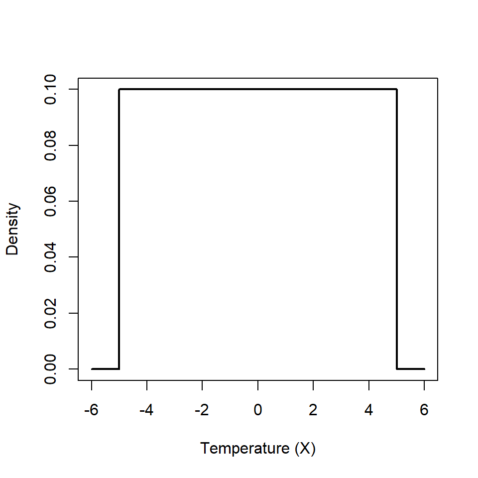
Figure 6.1: Probability density function for the temperature of a chemical reaction.

We can verify that \(f(x)\) is a PDF by checking that it satisfies the two conditions noted above. The limits in this example are [-5, 5] and we can see that \(f(x)=0.1\) on this interval which satisfies the first condition. The second condition requires a bit more work because we need to integrate the function between these limits (this is just for illustration):

\[\int _{-5}^{5} f(x)dx = \int _{-5}^{5} 0.1 dx = 0.1[x ]_{-5}^5 = 0.1(5 - -5) = 0.1 \times 10 = 1\]

Thus the area under the curve equals 1 and thus satisfies condition 2.

For a discrete random variable, the PMF defined the probability associated with a certain outcome and the sum of the probabilities for all outcomes equaled one. We have just seen that for a continuous random variable, integration of the PDF over all possible values also equals one (condition 2). Therefore, to obtain the probability associated with a range of specified values, we integrate the PDF over the range of the specified values - hence, equation ??.

For example, the probability that \(X\) is between -2.5 and 2.5 is given by:

\[Pr(-2.5 \le X \le 2.5) = \int_{-2.5}^{2.5} 0.1 \mathrm{d}x \]

\[ = 0.1[x]_{-2.5}^{2.5} = 0.1[2.5 - -2.5] = 0.1 \times 5 = 0.5\]

With a discrete random variable, the probability associated with a particular value (\(Pr(X=x)\)) can be calculated. This is not the same for a continuous random variable and only the probability for a range of possible values can be calculated. Think about a distribution of a continuous variable such as height (denoted by \(H\)); the probability that someone is between 165-166 cm can be found from

\[Pr(165 \le H \le 166) = \int_{165}^{166} f(h)dh \]

If the interval of interest reduces, say \(Pr(165 \le H \le 165.5)\), then it follows that the probability will also reduce. As the interval gets narrower the probability will also reduce until the interval is so precise that the probability is effectively zero and hence, the probability of a particular value is zero. Thus for continuous distributions, only intervals are considered.

6.2.2 Cumulative distribution function

The cumulative distribution function, (CDF), for a continuous random variable is the same as for a discrete random variable, i.e.  \[ F(x) = Pr(X \leq x) \]

However, while the calculation of the CDF involves summation for a discrete random variable it involves integration for a continuous random variable. For example, the probability that the temperature is less than 0 is given by:

\[ F(x) = Pr(X \leq 0) = \int_{-5}^{0} 0.1 \mathrm{d}x \]

\[ = 0.1[x]_{-5}^{0} = 0.1[0 - -5] = 0.1 \times 5 = 0.5 \]

This calculation is shown to illustrate how the probability is obtained. In practice, we will use R to do the calculations because integrating some of the specific distributions we will consider is a non-trivial task.

6.2.2.1 Doing this in R

As with the binomial distribution shown in the previous chapter, there are functions which can be used to calculate probabilities for a uniform distribution; not surprisingly, the functions have the suffix unif. To define a uniform function, the minimum and maximum values are required (in this example of a chemical reaction, these are -5 and 5, respectively).

# Create a range of values (make wider than limits of the distribution)
xvalues <- seq(-6, 6, by=0.01)
# Create a dataframe
results <- data.frame(x=xvalues)
# Calculate density specifying limits of distribution 
results$density <- dunif(x=results$x, min=-5, max=5) 
# Plot PDF
plot(results$x, results$density, type="l", xlab="x", ylab="Density")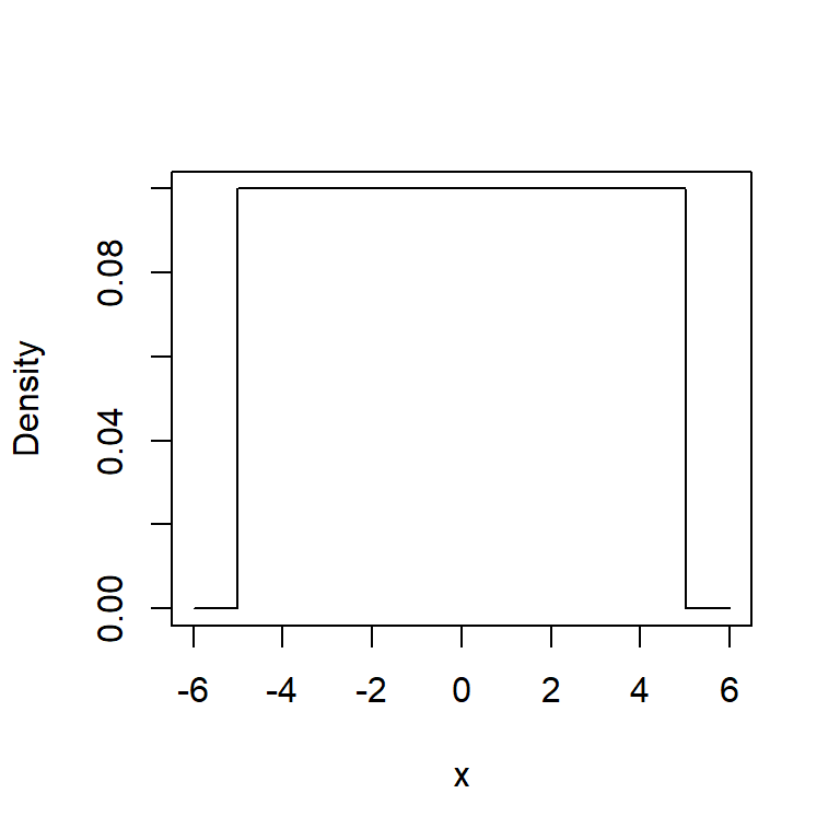

# Calculate CDF
results$CDF <- punif(q=results$x, min=-5, max=5)
# Plot CDF
plot(results$x, results$CDF, type="l", xlab="x", ylab="CDF")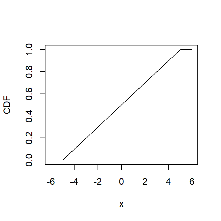

6.2.3 Expectation and variance

Similar to a discrete random variable, the expectation for a continuous random variable is like a weighted sum, but this time integration is required.

\[\begin{equation} E(X) = \int_{-\infty}^{\infty}xf(x)dx \end{equation}\]

Likewise the variance is given by,

\[\begin{equation} Var(X) = \int_{-\infty}^{\infty}(x - E(X))^2f(x)dx \end{equation}\]

which is equivalent to

\[\begin{equation} Var(X) = E(X^2) - [E(X)]^2 \end{equation}\]

Example In the chemical reaction, the expected value is given by

\[E(X) = \int_{-5}^{5} x0.1 dx\] \[ =0.1[\frac{x^2}{2}]_{-5}^{5} = \frac{0.1}{2}[25 - 25] = 0 \] Thus, the expected temperature in the chemical reaction is 0; this makes sense if we look at Figure 6.1 - it is the central value of \(X\).

6.3 Special continuous distributions

An example of a uniform distribution has just been introduced. There are several other distributions that will crop up later in the course, specifically the normal, \(t\) and \(F\) distributions.

These theoretical distributions are characterised by parameters which describe the location, scale and shape of the curve. In general, the properties of these parameters are as follows:

• location fixes the mid point of the distribution (or the lower point, depending on the distribution) on the number scale or \(x\)-axis (e.g. is the midpoint of the distribution at 10 or 100 etc.),

• scale determines length of the \(x\)-axis (e.g. how spread out the distribution is along the \(x\)-axis),

• shape allows the curve to take a variety of shapes, perhaps shifting or stretching the distribution along the \(x\)-axis.

Not all distributions have all these parameters and the distributions described in this document are characterised by only one or two parameters. The normal distribution is used for many applications and so we look at this distribution in detail.

6.3.1 Normal distribution

A normally distributed random variable \(X\) is defined by two parameters, \(\mu\) and \(\sigma^2\), where \(\mu=E(X)\) and \(\sigma^2=Var(X)\). This can be written more concisely as \(X \sim N(\mu, \sigma^2)\). The normal distribution is symmetrical and the parameter \(\mu\) defines the centre of the distribution and \(\sigma^2\) defines the spread.

How different values of \(\mu\) and \(\sigma^2\) affect the shape of the distribution can be seen in Figure 6.2. Note that, because of condition 2, the area under all the curves is one and so there is a trade-off between the maximum density of the distribution and how spread out the distribution is along the \(x\)-axis.

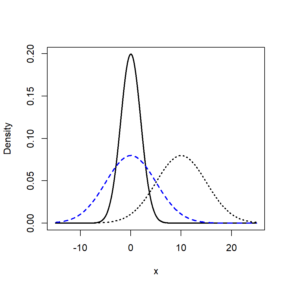
Figure 6.2: Examples of normal distributions with different values of \(\mu\) and \(\sigma^2\); \(N(0,4)\) (black line), \(N(0,25)\) (blue dashes), \(N(10, 25)\) (black dots).

The probability distribution function for the normal distribution is given by:

\[\begin{equation} f(x; \mu, \sigma) = \frac{1}{\sqrt{2\pi\sigma^2}}e^{[\frac{-1}{2\sigma^2}(x-\mu)^2]} \end{equation}\]

Normal distributions have some useful properties (which we make use of in future chapters):

• they are symmetric about the mean and median (which are equal)

• 68% of observations are within \(\pm 1 \times \sigma\) of \(\mu\) (i.e. 68% of the area is within the interval \(\mu-\sigma\) and \(\mu + \sigma\))

• 95% of observations are within \(\pm 1.96 \times \sigma\) of \(\mu\)

• 99% of observations are within \(\pm 2.58 \times \sigma\) of \(\mu\)

This can be seen in Figure 6.3.

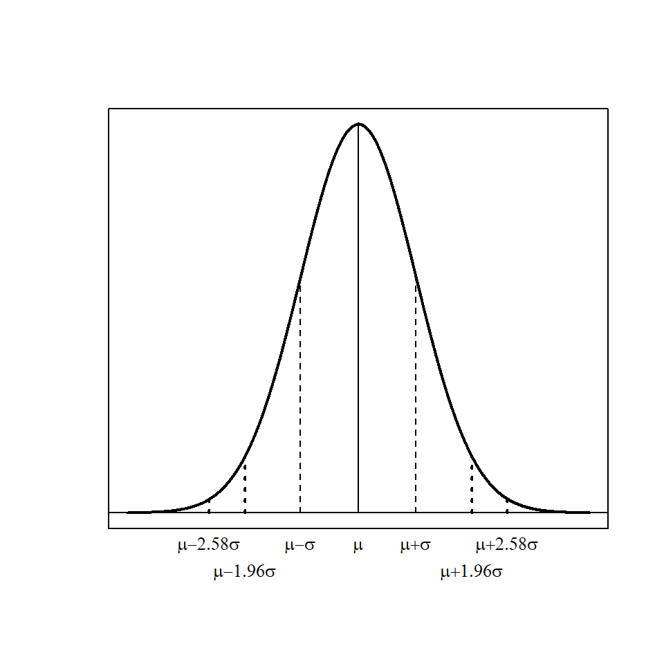
Figure 6.3: Normal distribution, \(N(\mu, \sigma^2)\); 68% of the values are within 1 standard deviation of \(\mu\) (dashed lines), 95% of the values are within 1.96 standard deviations (dotted line) and 99% within 2.58 standard deviations.

6.3.1.1 Doing calculations in R

Many measurements will have empirical frequency distributions that are normal, or nearly normal. This can be helpful in that we can then use this information to find out about the population, given knowledge of \(\mu\) and \(\sigma\). Remember that condition 2 specifies that the area under \(f(x)\) for all possible values of \(X\) is equal to one (there is an equivalent condition for discrete random variables), hence the area of different intervals can inform us about the probability of these intervals.

For example, assume the distribution of womens heights (\(X\)) is approximately normal with a mean 160cm and standard deviation 6cm (i.e. \(X \sim N(160, 6^2)\)). We want to find the probability that a randomly chosen woman is smaller than 150cm (\(Pr(X \le 150)\)) and this is given by the area under the curve less than 150 cm (Figure 6.4).

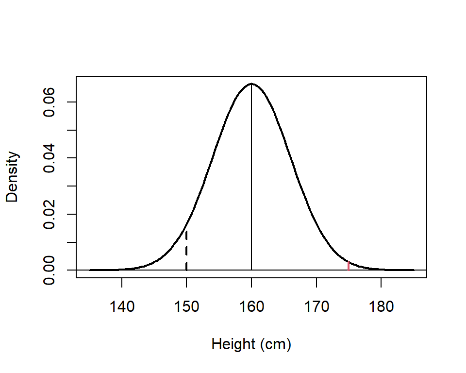
Figure 6.4: Plot of the distribution for womens height, \(N(160, 6^2)\). The dashed line is at 150 cm and the red line is at 175 cm.

As we have seen, we can find this from the cumulative distribution function and we can use R to do the calculations:

# Specify parameters
mu <- 160 # Mean
sigma <- 6 # Standard deviation
# CDF - area under the curve less than q
pnorm(q=150, mean=mu, sd=sigma, lower.tail=TRUE)

[1] 0.04779035

The probability is 0.04779, hence, approximately 4.78% of women will be less than 150 cm.

What about the probability that a randomly chosen women will be greater than 175 cm (i.e. \(Pr(X > 175)\))? In this case we want the area under the curve for values greater than 175 (red line in Figure 6.4). Again we can use R to do the calculations and there are two possible options. The first calculation uses the complement rule and the CDF. Hence,

\[Pr(X > 175) = 1 - Pr(X \le 175)\] In R, the command is:

1 - pnorm(q=175, mean=mu, sd=sigma)

[1] 0.006209665

We can be somewhat casual about \(\le\) and \(<\) (and also \(\ge\) and \(>\)) signs because as we have seen the \(Pr(X=a) = 0\). (Note, this does not apply to discrete random variables.)

R provides an alternative method to obtain \(Pr(X > 175)\), if an additional argument is specified in the pnorm function. By default, the area to the left of a specified value (q), or the lower tail (i.e. the CDF), is returned by pnorm. Specifying the argument lower.tail=FALSE will return the area to the right of q (the upper tail), hence, we can obtain the relevant probability directly:

# Area under curve greater than q
pnorm(q=175, mean=mu, sd=sigma, lower.tail=FALSE)

[1] 0.006209665

These functions make calculating probabilities relatively straight forward, for example, we can find the probability a women is between 148 and 172 cm, i.e. \(Pr(148 \le X \le 172)\).

# Area under curve in interval 148 to 172
area172 <- pnorm(q=172, mean=mu, sd=sigma, lower.tail=TRUE)
area148 <- pnorm(q=148, mean=mu, sd=sigma, lower.tail=TRUE)
area172 - area148

[1] 0.9544997

Why is this probability not surprising? Hint, how many values of \(\sigma\) are these limits away from the mean?

The interval 148 to 172 is \(\mu \pm 2 \sigma\) and we know that for a normal distribution, 95% of the distribution falls within 1.96 standard deviations of the mean. Hence, we would expect the probability to be very close to 95%.

6.3.2 Standard normal distribution

A special case of the normal distribution is the standard normal distribution where \(\mu=0\) and \(\sigma^2=1\). The PDF is simpler:

\[\begin{equation} f(x; \mu, \sigma) = \frac{1}{\sqrt{2\pi}}e^{\frac{(x - \mu)^2}{2}} \end{equation}\]

The standard normal distribution is very useful because any given normal distribution can be transformed to a standard normal PDF by converting the normal random variables to standard units. This process, called standardization, is simply

\[\begin{equation} Z = \frac{X - \mu}{\sigma} \end{equation}\]

A random variable from a standard normal distribution is often denoted by \(Z\), i.e \(Z \sim N(0, 1)\). Sometimes the term ‘normalisation’ is used instead of standardisation but they refer to different transformations: normalisation usually means to scale the data values so they they lie between 0 and 1; standardisation transforms the data to have a mean 0 and standard deviation of one.

Example Assume that IQ (intelligent quotient) is distributed as \(N(100,15^2)\). What is the IQ for someone at the 99th percentile i.e. what is \(q\) such that \(Pr(X \le X q)=0.99\)?

We can find this value using the CDF function in R.

qnorm(p=0.99, mean=100, sd=15)

[1] 134.8952

Alternatively, we can find the 99th percentile for the standard normal, then multiply by \(\sigma\) and add \(\mu\) i.e. 

\[ X = Z \sigma + \mu\]

# Use standard normal and transform
qnorm(p=0.99, mean=0, sd=1)*15 + 100

[1] 134.8952

Thus, the IQ for someone in the 99th percentile will be nearly 135.

6.3.3 Simple transformations of random variables

Sometimes we may wish to consider transformations of random variables other than standardisation; for example a variable has been measured in some unit (e.g. inches) and we want to transform it to another unit of measurement (e.g. centimetres) and find the expected value in the new units of measurement.

There are some simple rules that we can apply in these cases which apply for both continuous and discrete random variables.

6.3.3.1 Adding and multipling by a constant

Let \(X\) be a random variable and let \(Y\) be some function of \(X\) that involves either the multiplication of a constant \(a\), the addition of some constant \(b\) or indeed both. The expected value of \(Y\), \(E(Y)\), can then be found using these simple rules:

• \(Y = aX\) and \(E(Y) = aE(X)\).

• \(Y = X + b\) and \(E(Y) = E(X) + b\).

• \(Y = aX + b\) and \(E(Y)= aE(X) + b\).

Example The expected temperature at a particular location was \(10^o\)Celsius. What is the expected value in Fahrenheit?

The conversion from Celsius (\(C\)) to Fahrenheit (\(F\)) is \[ F = 1.8C + 32\] Therefore, the expected value in Fahrenheit is given by:

\[E(F) = 1.8E(C) + 32 = 1.8 \times 10 + 32 = 50\] Hence, the expected value in Fahrenheit is 50\(^o\).

What about the variance of a simple transformation? Similar rules to those for the expectation also apply:

• \(Y = aX\) then \(Var(Y)= a^2Var(X)\)

• \(Y = X + b\) then \(Var(Y)= Var(X)\)

• \(Y = aX + b\) then \(Var(Y)= a^2Var(X)\).

If a constant is added to, or subtracted from, \(X\), then the expected value is shifted by this amount but the variability is unchanged. Conversely, if a variable is multiplied by a constant, the expected value is also multiplied by the constant and the variance is multiplied by the constant squared.

We can illustrate these rules empirically by generating some random data. Here we generate data for a variable \(X \sim N(\mu=20, \sigma^2=9)\).

# Set seed
set.seed(1234)
# Generate 100 random values from a normal distribution (with mean 20 and sd 3)
X <- rnorm(n=100, mean=20, sd=3)
# Expected value and variance of X
mean(X)

[1] 19.52971

var(X)

[1] 9.07947

The transformation is specified \(Y = 2X + 5\) and so we create \(Y\) and then obtain the mean and variance using the usual R functions.

# Let Y = 2X + 5
Y <- (2 * X) + 5
# Expected value and variance of Y
mean(Y)

[1] 44.05943

var(Y)

[1] 36.31788

Thus, the mean of \(Y\) is 44.06 and the variance is 36.32. Now, we use the rules above to obtain the mean and variance of \(Y\) from the mean and variance of \(X\), \(E(X)\) and \(Var(X)\):

# Use rules to obtain expected value of y
(2*mean(X)) + 5

[1] 44.05943

# and variance
4*var(X)

[1] 36.31788

The same values were obtained as before; the other rules can be similarly demonstrated.

6.3.3.2 Adding random variables

Sometimes we may wish to consider a transformation including two random variables, \(X\) and \(Y\). In this case, the expected value for adding the variables, (\(X + Y\)), is given by:

\[\begin{equation} E(X + Y) = E(X) + E(Y) \end{equation}\]

Similarly, the expected value for subtracting the variables, \((X-Y)\), is given by:

\[\begin{equation} E(X - Y) = E(X) - E(Y) \end{equation}\]

If we assume that \(X\) and \(Y\) are independent, the variances can simply be added to obtain both \(Var(X+Y)\) and \(Var(X-Y)\):

\[\begin{equation} Var(X+Y) = Var(X-Y) = Var(X) + Var(Y) \end{equation}\]

More complicated transformations can be considered using previous rules, for example,

\[Z = a + bX + cY\] Hence,

\[\begin{equation} E(Z) = a + bE(X) + cE(Y) \label{rvtransexp} \end{equation}\]

and, similarly if \(X\) and \(Y\) are independent, the variance is given by

\[\begin{equation} Var(Z) = b^2Var(X) + c^2Var(Y) \end{equation}\]

Example A time-and-motion study measures the time required for an assembly line worker to perform two successive repetitive tasks. The data showed that the time required to position a part on an automobile chassis varied from car to car with mean 11 seconds and standard deviation 2 seconds. The time required to attach the part to the chassis also varied, with mean 20 seconds and standard deviation 4 seconds. What is the expected combined time for positioning and attaching the part?

To answer this, let \(X\) represent the time to position the part and \(Y\) represent the time to attach the part. The expected total time taken to position and attach a part, \(X+Y\), is given by:

\[ E(X+Y) = E(X) + E(Y) = 11 + 20 = 31 \textrm{ seconds}\]

The time-and-motion study finds that the times required for the two steps are independent, i.e. the time to attach a part is not affected by the time taken to position the part. What is the standard deviation for the time to position and attach the part?

\[V(X+Y) = V(X) + V(Y) = 2^2 + 4^2 = 20 \]

\[SD(X+Y) = \sqrt{V(X+Y)} = \sqrt{20} = 4.47 \textrm{ seconds}\]

So far we have considered variables that are independent but if this is not the case, then we need to take into account how closely related they are.

6.3.3.3 Covariance and correlation

If \(X\) and \(Y\) are not independent, then the covariance, a measure of the degree of association or similarity, of \(X\) and \(Y\), needs to be taken into account when calculating the variance:

\[\begin{align} Var(X+Y) = Var(X) + Var(Y) + 2Cov(X,Y) \\ Var(X-Y) = Var(X) + Var(Y) - 2Cov(X,Y) \end{align}\]

The covariance is explored further but first another useful rule theorem is required.

If two independent random variables are multiplied, the expected value of the product is the product of the expected values, or more succinctly:

\[\begin{equation} E(XY) = E(X)E(Y) \end{equation}\]

The covariance between two random variables \(X\) and \(Y\) is:

\[\begin{align} Cov(X,Y) = E[(X-E(X))(Y-E(Y))] \\ = E(XY) - E(X)E(Y) \end{align}\]

Independent random variables have zero covariance.

A related measure is the correlation coefficient, \(\rho\), which measures the linear relationship between two variables:

\[\begin{equation} \label{corcoeffeqn} \rho = \frac{Cov(X,Y)}{\sqrt{Var(X)Var(Y)}} \end{equation}\]

Correlation is explored further in Chapter 13.2 and so it is not expanded on here, except to say that \(\rho\) (or denoted by \(r\) for a sample) can take values between -1 and 1 (inclusive) and when \(\rho=1\), there is a positive linear relationship between \(X\) and \(Y\), when \(\rho=-1\), there is a negative relationship between \(X\) and \(Y\) and when \(\rho=0\), there is no relationship between \(X\) and \(Y\).

We can rearrange equation ?? so that

\[Cov(X,Y) = \rho \sqrt{Var(X)Var(Y)}\]

and then substitute into equations, such that

\[\begin{align} Var(X+Y) = Var(X) + Var(Y) + 2\rho \sqrt{Var(X)Var(Y)} \\ Var(X-Y) = Var(X) + Var(Y) - 2\rho \sqrt{Var(X)Var(Y)} \end{align}\]

Example How would the standard deviation change, if the time taken to position and attach a part were dependent, with a correlation coefficient of 0.8?

\[Var(X+Y) = Var(X) + Var(Y) + 2\rho\sqrt{Var(X)Var(Y)}\]

\[ =2^2 + 4^2 + 2 \times 0.8 \times \sqrt{2^2 \times 4^2} = 32.8\] \[SD(X+Y) = \sqrt{32.8} = 5.73 \textrm{ seconds}\] Q6.1 Using the time-and-motion study described in the example, the variation in the worker’s performance is reduced by better training, and hence the standard deviations of positioning and attaching the parts has decreased. Will this decrease change the expected value of the combined steps, if the mean times for the two steps remain as before?

Q6.2 A company makes a profit of 2,000 on each military unit sold and 3,500 on each civilian unit. Thus the profit is from military units is 2,000\(X\) where \(X\) is the number of military units sold; similarly, the profit from civilian units is 3,500\(Y\), where \(Y\) is the number of civilian units sold. The expected number of military units to be sold is 5,000 and the expected number of civilian units to be sold is 445. Using this information answer the following questions.

a. What is the expected profit on military units?

b. What is the expected total profit for military and civilian units?

c. What is the expected difference in profit between military and civilian units?

d. Assuming that the number of military and civilian units sold are independent, describe how to calculate the variance of the total profit. Will this be different to the variance of the difference calculated in part c?

Q6.3 Planks of wood are cut into two sizes, short and long. The length (in metres) of the short planks has a \(N(0.5, 0.01)\) distribution and the length of the long planks has a \(N(1.5, 0.0625)\) distribution. It was found that one short plank and two long planks placed end to end were required to make one floorboard.

a. What is the mean length of floorboards?

b. Assuming that the two lengths of plank are independent, what is the variance of the floorboard.

c. What is the probability that the floorboard will be too long for a room 4 metres in length?

6.4 Summary

There are analogous functions to the PMF and CDF for continuous random variables, the main difference is that we need to integrate under the curves to obtain probabilities, expected values and variances rather than summation.

The normal and standard normal distributions have been described in detail. These distributions crop up frequently in statistics; other distributions considered in following chapters are the \(t\) and \(F\).

Random variables can be transformed in various ways and there are simple rules which can be applied to obtain the expected values and variances of these transformations.

6.4.1 Learning outcomes

In this chapter, you have learnt definitions for the

1. PDF and CDF

2. expectation and variance

for continuous random variables. The normal and standard normal distributions have been described in detail and rules for obtaining the expected value and variances for simple transformations of random variables have been illustrated.

6.5 Answers

Q6.1 No. Changing the standard deviations will not change the means.

Q6.2 a. Consider \(X_T = 2000X\), then using \[E(X_T) = 2000E(X) = 2000 \times 5000 = 10000000\]

the expected profit is \(\pounds 10,000,000\).

Q6.2 b. The expected total profit is obtained from

\[ E(2000X+3500Y) = 2000E(X) + 3500E(Y) = 2000 \times 5000 + 3500 \times 445 = 11557500 \] Hence, the expected total profit is £\(11,557,500\).

Q6.2 c. The expected difference in profits between military and civilian sales can be calculated from

\[E(2000X - 3500Y) = 2000E(X) - 3500E(Y) = 2000 \times 5000 - 3500 \times 445 = 8442500\] Thus, the expected difference in profits is £8,442,500.

Q6.2 d. The variance for \(2000X\) units is given by \(Var(2000X) = 2000^2Var(X)\) and similarly the variance for \(3500Y\) is \(Var(3500Y) = 3500^2Var(Y)\).

If the units sold for military and civilian use are independent, then the variances can be added to calculate the variance of the total profit:

\[Var(2000X + 3500Y) = 2000^2Var(X) + 3500^2Var(Y)\] The variance will be the same for the difference in profits.

Q6.3 Let \(X\) represent the short planks and \(Y\) represent the long planks and so a floorboard is made up of \(F = X + Y1 + Y2\).

Q6.3 a. Using equation ??, let \(a=0\), \(b=1\) and \(c=2\), \[E(F) = 1 \times E(X) + E(Y1) + E(Y2) = 0.5 + 1.5 + 1.5 = 3.5\] The expected length of a floorboard is 3.5m.

Q6.3 b. Similarly, the variance is given by \[Var(F) = 1 \times Var(X) + Var(Y1) + Var(Y2) = 0.01 + 0.0625 + 0.065 = 0.135\] Q6.3 c. The probability \(Pr(F > 4)\) is required, where \(F \sim N(3.5, 0.26)\). R can be used to find this probability with the pnorm command. There are two equivalent commands:

Using \(1 - Pr(X \le 4)\)

1 - pnorm(q=4, mean=3.5, sd=sqrt(0.26))

[1] 0.1633998

Alternatively,

pnorm(q=4, mean=3.5, sd=sqrt(0.26), lower.tail=FALSE)

[1] 0.1633998

Therefore, the probability that a floorboard is greater than 4 m is 0.163.