Chapter 9 Analysis of Variance
The analysis of variance is not a mathematical theorem, but rather a convenient method of arranging the arithmetic.
R. A. Fisher, 1934.
9.1 Introduction
Previously we have considered the comparison of two groups. In this chapter, we consider the comparison of more than two group means using a procedure called analysis of variance (generally called ANOVA). ANOVA indicates whether at least one group is different from at least one other group mean. To identify where those differences lie, we need to then consider each of the pairwise comparisons but taking into account that we are making several comparisons.
In this chapter we will consider:
- the number of comparisons when there are more than two groups,
- determining if there is a difference in the group means and where any differences might lie,
- checking test assumptions and
- alternative methods if the assumptions are not valid.
9.2 Multiple comparisons
We start with a motivating example; a sample of plants have been grown in three different growing mediums and the amounts of various chemical elements in a leaf from each plant have been obtained. It was felt that the chemical composition of the plants was specific to growing medium and, if so, this may help identify where the plants were grown. The growing mediums, or groups, were classified as B, N and P and here, we are interested in whether the mean titanium levels differ between the three groups (Figure 9.1).
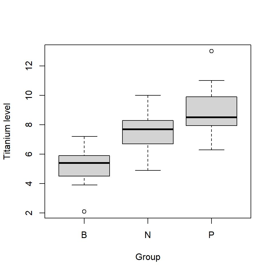
Figure 9.1: Distributions of titanium levels in three groups.
In Figure 9.1 we see that there is substantial overlap in the values between the three groups and so we will require formal methods to determine if the underlying groups means are the same, or if there is a real difference (beyond sampling variability). We could conduct a series of two sample \(t\) tests and compare B with N, B with P and N and P. However, the more tests we undertake, i.e. when making a series of comparisons, the higher the chance of drawing a false conclusion.
9.2.1 Type I and Type II error
When using a fixed significance level to draw a conclusion, the significance level, \(\alpha\) is the associated error rate - the probability of rejecting the null hypothesis when it is, in fact, true. For example, a significance level of 5% (\(\alpha=0.05\)) means that there is a 5% chance of rejecting the null hypothesis when it should not be rejected (e.g. there is no difference between means). This is known as a Type I error. The converse error also exists, called a Type II error.
Type I error - rejecting the null hypothesis when it is true (false positive)
Type II error - not rejecting the null hypothesis when it is false (false negative)
Table 9.1 should help with understanding.
| Outcome of test | \(H_0\) True | \(H_0\) False |
|---|---|---|
| Reject \(H_0\) | Type I Error | Correct decision |
| Fail to reject \(H_0\) | Correct decision | Type II Error |
In comparing each pair of groups, there is a Type I error associated with each test and the Type I error compounds every time we do an additional test. The error rate over all possible pairwise comparisons is then no longer 5% and increases the chance of drawing false conclusions. We come back to this later in the chapter but essentially what we need is one test that compares all group means simultaneously; we do this using one-way Analysis of Variance.
9.3 ANalysis Of VAriance (ANOVA)
We want to test for differences in means between three or more groups. The null hypothesis will be that the group means are the same and the alternative hypothesis will be that, at least, one mean is different from at least one other mean.
Example The null hypotheses to compare the mean titanium levels in three groups, B, N and P is:
\[ H_0: \mu_{\textrm{B}} = \mu_{\textrm{N}} = \mu_{\textrm{P}} \] The alternative hypothesis is usually specified as
\[H_1: \textrm{at least one mean is different from one of the other means}\] because specifying all the options is rather long-winded, i.e. \(\mu_{\textrm{B}} = \mu_{\textrm{N}} \ne \mu_{\textrm{P}}\) or \(\mu_{\textrm{B}} \ne \mu_{\textrm{N}} = \mu_{\textrm{P}}\) or \(\mu_{\textrm{B}} \ne \mu_{\textrm{P}} = \mu_{\textrm{N}}\) or \(\mu_{\textrm{B}} \ne \mu_{\textrm{N}} \ne \mu_{\textrm{P}}\).
If \(H_0\) is true, we would expect the group means to be similar and any observed differences between the sample means is due to sampling variation only. However, as we have seen comparing two groups, detecting differences between group means depends on the variability associated with each group. If there are no differences between means (i.e. the null hypothesis is true) then any differences between the group means are likely to be small compared with the within group variability (Figure 9.2).
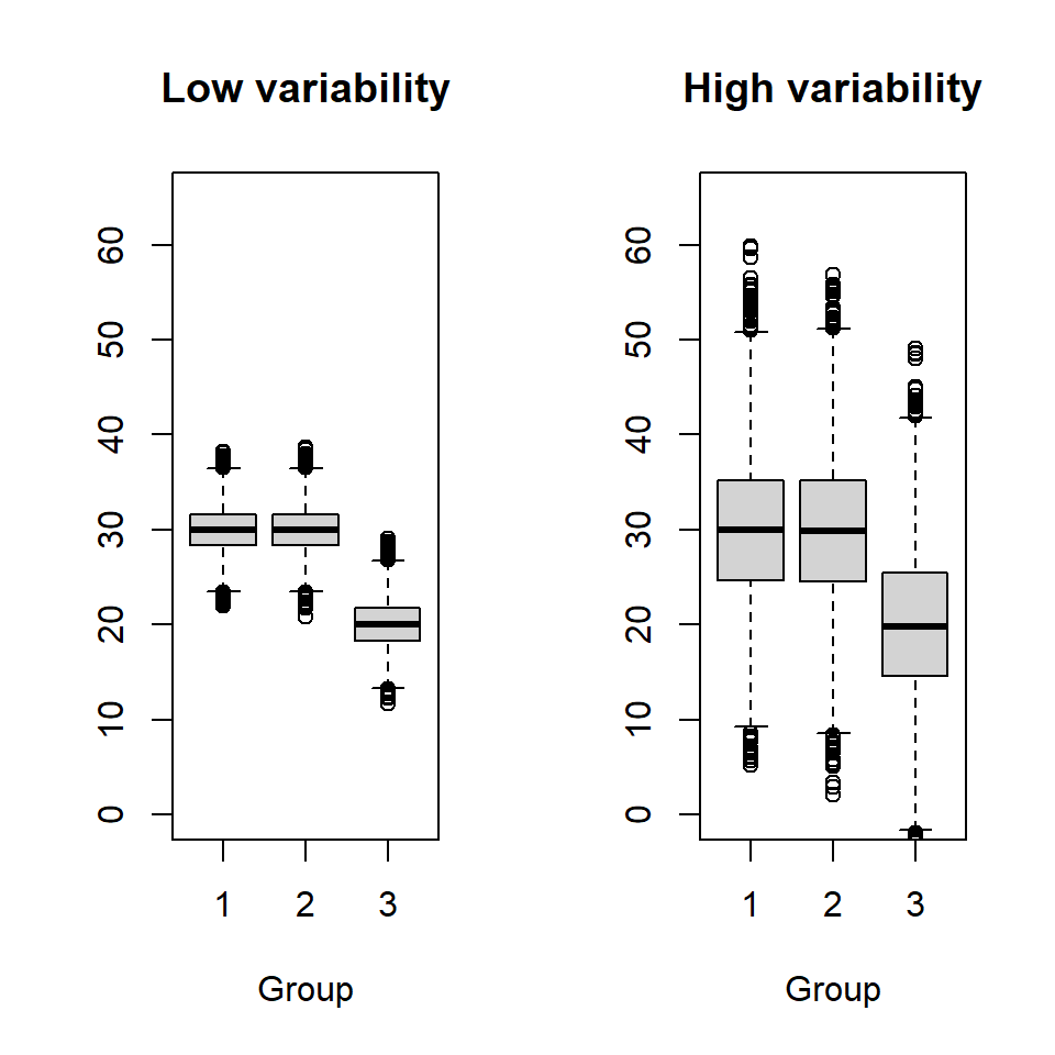
Figure 9.2: Illustration of between and within group variability; the mean for groups 1 and 2 is 30 and the mean for group 3 is 20. The standard deviation is 2.5 in the left plot and 8 in the right.
The ANOVA procedure explicitly compares the ‘between’ and ‘within’ group variability to test \(H_0\). This is done using an \(F\) test statistic.
9.3.1 \(F\) test statistic for ANOVA
The \(F\) test statistic for ANOVA is the ratio of the variability between groups (\(s_G^2\)) and the variability within groups (\(s_W^2\)):
\[f_0=\frac{s^2_G}{s^2_W}\]
The numerator, \(s^2_G\), represents the difference between each group mean and the overall mean (combined across groups). It will be large if there are large differences between the group means:
\[s^2_G=\frac{\sum_{i=1}^{k} n_i (\bar{x}_{i}-\bar{x}_{.})^2}{k-1}= \frac{SS_G}{k-1}\]
where
- \(k\) is the number of groups,
- \(n_i\) is the sample size for group \(i\) and \(i=1, ..., k\),
- \(\bar{x}_{i}\) is the sample mean for group \(i\), and
- \(\bar{x}_{.}\) is the sample mean across all groups combined.
The denominator, \(s^2_W\), represents the variability within groups (via \(s^2_i\)) weighted by sample size within groups. It will be large if the data vary a great deal within groups (Figure 9.2, right hand plot):
\[s^2_W = \frac{\sum_{i=1}^{k}(n_i-1)s_i^2}{n_{tot} - k} = \frac{SS_W}{n_{tot} - k}\]
- where \(s_i^2\) is the sample variance for group \(i\), and
- \(n_{tot}\) is the total number of observations across all groups.
If \(H_0\) is true, \(f_0\) should be small - differences between means are small compared with the spread within groups. If \(H_0\) is false, \(f_0\) should be large - differences between means will be large compared to the spread within groups. Evidence against \(H_0\) is provided by values of \(f_0\) which would be unusually large when \(H_0\) is true. How large is large?
Deciding if a test statistic is typical under the null hypothesis, we compare the test statistic with a reference distribution; in this case, the \(F_{(df_1,df_2)}\) distribution, where \(df_1=k-1\) and \(df_2=n_{tot}-k\) is used. This distribution is also used to obtain an exact \(p\)-value for the test; we will use R for this in general (although there are tables where critical values can be looked up). Before looking at the \(F\) distribution, we examine how \(f_0\) is calculated. As with \(p\)-values, we will generally use R to calculate \(f_0\), however, it is useful to see how it is calculated and presented.
9.3.2 Calculating an ANOVA table
A convenient way to compile all the values for an \(F\) test statistic is to compile an ANOVA table (Table 9.2). The variability observed in the data is partitioned into the pattern, or signal, which can be explained by the different groups and then what is left over, called errors or residuals. Residuals will crop up later when regression models are described. In fact with ANOVA, we are fitting a model, it is just that the explanatory variable is a nominal variable.
| Source of variation | df | Sum Sq | Mean Sq | \(F\) value |
|---|---|---|---|---|
| Between groups | \(k-1\) | \(SS_G\) | \(s_G^2\) | \(f_0\) |
| Residuals | \(n_{tot}-k\) | \(SS_W\) | \(s_W^2\) | |
| ————— | ————– | ——— | ———- | – |
| Total | \(n_{tot}-1\) |
The completed ANOVA table to test for differences between the mean titanium level in groups B, N and P is given in Table 9.3.
| Source of variation | df | Sum Sq | Mean Sq | \(F\) value |
|---|---|---|---|---|
| Between groups | 2 | 118.60 | 59.30 | 28.31 |
| Residuals | 43 | 90.06 | 2.09 | |
| ————— | ————– | ——— | ———- | – |
| Total | 45 |
To illustrate the calculations, the number of observations, sample means and standard deviations are required for each group and also these values overall groups (Table 9.4).
| GM | n | Mean | SD |
|---|---|---|---|
| B | 13 | 5.1 | 1.318 |
| N | 9 | 7.58 | 1.622 |
| P | 24 | 8.85 | 1.447 |
| Total | 46 | 7.54 | 2.153 |
Each component of the table is calculated as follows:
\[\begin{equation}\label{} \begin{split} SS_G & = \sum_{i=1}^{k} n_i (\bar{x}_{i.}-\bar{x}_{..})^2 \\ & = 13(5.10 - 7.54)^2 + 9(7.58 - 7.54)^2 + 24(8.85 - 7.54)^2 \\ & = 118.60 \end{split} \end{equation}\]
\[s^2_G = \frac{SS_G}{k-1} = \frac{118.60}{3-1} = 59.30 \]
\[\begin{equation} \begin{split} SS_W & = \sum_{i=1}^{k}(n_i-1)s_i^2 \\ & = (13-1)1.318^2 + (9-1)1.622^2 + (23-1)1.447^2 \\ & = 88.16 \end{split} \end{equation}\]
\[s^2_W = \frac{SS_W}{n_{tot}-k} = \frac{90.06}{46 - 3} = 2.09\] Finally,
\[f_0 = \frac{s^2_G}{s^2_W} = \frac{59.307}{2.09} = 28.31\]
Hence, the test statistic is 28.31. To decide whether this is large, we compare it to the \(F_{(df_1,df_2)}\) distribution.
9.3.3 \(F\) distribution
The \(F\) distribution (named in honour of R. A. Fisher) is a continuous distribution. It is defined by two parameters, \(F_{df_1,df_2}\), where,
- \(df_1 = k - 1\)
- \(df_2 = n_{tot} - k\).
The \(F\) distribution can take on a variety of shapes but cannot have negative values. Figure 9.3 shows some examples of shapes and you can also explore the shape changes yourself in Figure 9.4.
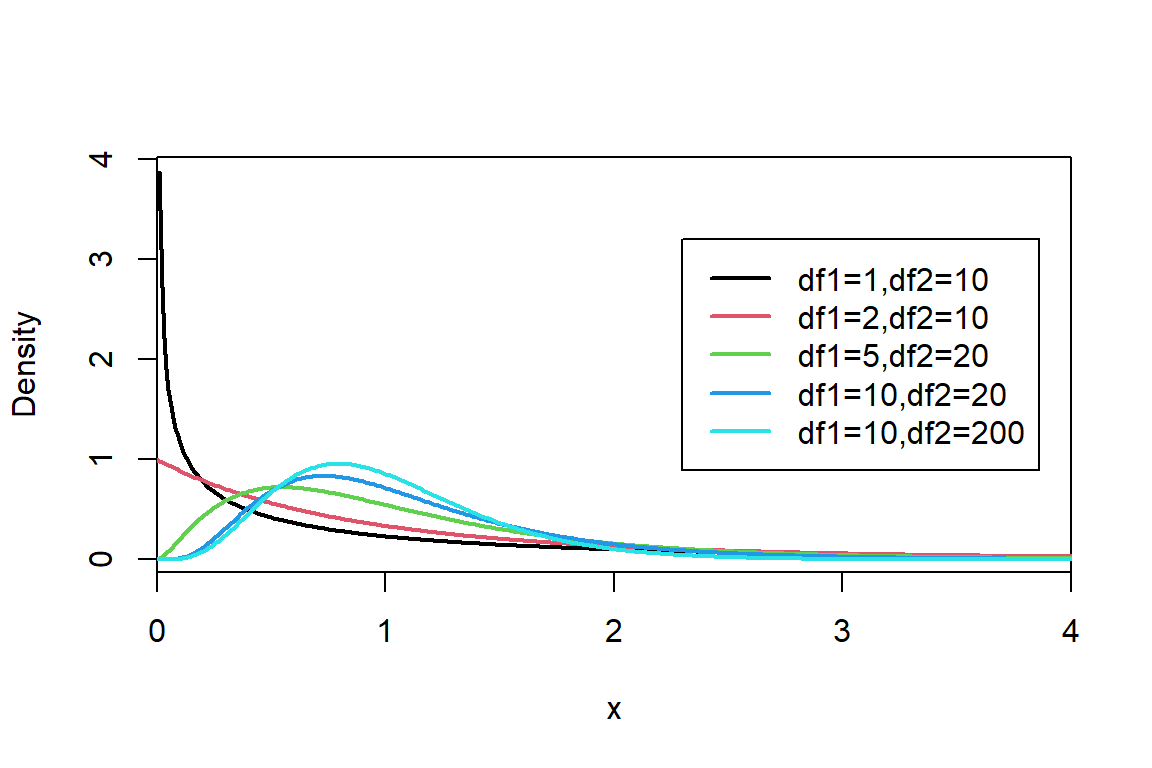
Figure 9.3: The probability density function of \(F_{df1,df2}\) distribution for different values of the parameters \(df1\) and \(df2\).
Figure 9.4: Visualising the \(F\) distribution. You can see a live version by clicking here
In our example, \(df_1=2\) and \(df_2=43\) and this distribution is shown in Figure 9.5. We can see that the density (on the \(y\)-axis) at a value of about 6 on the \(x\)-axis is pretty much zero. Our test statistic is 28.31, hence the probability of obtaining a value as large and larger than this (i.e. \(Pr(f \ge 28.31)\) where \(f \sim F_{2,43}\)) is going to be very, very small; in fact the \(p\)-value is \(<0.0001\). This indicates that it is very unlikely to obtain a value as large, or larger, than 28.31 when the group means are the same. We reject \(H_0\) and have strong evidence that at least one of the group means is different to one of the other means.
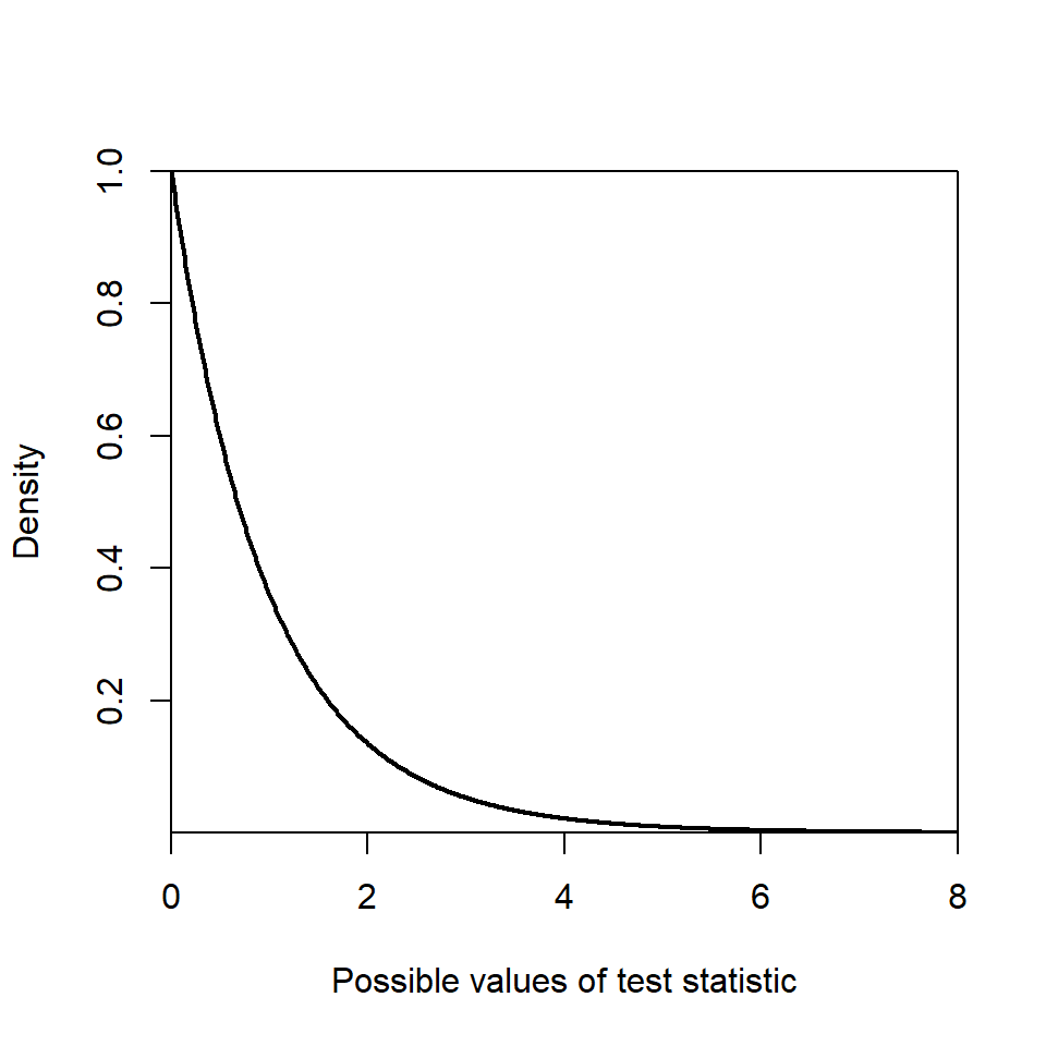
Figure 9.5: Reference distribution, \(F_{2,43}\) distribution.
9.3.4 Doing this in R
Fortunately, R removes the hard work and does all the calculations, however, to make sense of the output created by the aov function, and create a neat ANOVA table, the summary function is used.
# Fit ANOVA
plant.aov <- aov(Ti ~ Group, data=plant)
# Display ANOVA table
summary(plant.aov)
Df Sum Sq Mean Sq F value Pr(>F)
Group 2 118.60 59.30 28.31 1.43e-08 ***
Residuals 43 90.06 2.09
---
Signif. codes: 0 '***' 0.001 '**' 0.01 '*' 0.05 '.' 0.1 ' ' 1The asterisks give a visual indication of the significance level; in this case the three asterisks (***) indicate that the \(p\)-value is between 0 and 0.001.
One thing to note is that the \(p\)-value is only associated with the upper tail. Hence, if we want to calculate the exact \(p\)-value, the upper tail has to be specified in the function to obtain the \(p\)-value, or indeed if we want to obtain a critical value.
# Exact p-value
pf(q=28.31, df1=2, df2=43, lower.tail=FALSE)
[1] 1.429293e-08# Critical value, testing at a significance level of 5%
qf(p=0.05, df1=2, df2=43, lower.tail=FALSE)[1] 3.21448The critical value, testing at a significance level of 5%, is 3.21 - our test statistic (\(f_0\)=28.31) is much larger than this, hence, leading us to the same conclusion.
Q9.1 A consumer organisation was interested in comparing the price of petrol (pence per litre) in four different locations classified as city, motorway, rural and town. Prices at ten petrol stations, selected at random for the four locations, were recorded; a summary of the results are provided below.
| Location | n | Mean | SD |
|---|---|---|---|
| City | 10 | 135.4 | 5.52 |
| Motorway | 10 | 143.6 | 3.84 |
| Rural | 10 | 140.4 | 6.43 |
| Town | 10 | 133 | 7 |
| Total | 40 | 138.1 | 7 |
a. Describe the null and alternative hypotheses to be tested.
b. Complete the ANOVA table to calculate the \(F\) test statistic.
c. A critical value, testing at a significance level of 5%, for the reference \(F\) distribution is given below. What do you conclude regarding the mean prices between locations?
qf(p=0.05, df1=3, df2=36, lower.tail=FALSE)[1] 2.8662669.3.5 Assumptions
In order for the \(F\) test results to be valid, we need the following assumptions to be met:
- Independence: the data are sampled independently,
- Normality: the data for each group appears to have come from a Normal distribution,
- Constant spread: the underlying standard deviations for each group appear to be equal.
ANOVA is reasonably robust to departures from the ‘constant spread’ and ‘Normality’ assumptions, however, the ‘independence’ assumption is critical for valid results. As a conservative rule of thumb, ANOVA should give reliable results if the largest standard deviation of the groups is no larger than twice the smallest standard deviation of the groups.
Example We can check these assumptions for the ANOVA we have conducted on the plant data. Within each group, different plants were measured for titanium levels and without knowing further details of the data collection, we assume the values are independent. The other assumptions can be tested more formally.
9.3.5.1 Checking constant spread
Table 9.4 indicates that the standard deviations are similar in each group based on the rule of thumb - the smallest is 1.318 and the largest is 1.622. Levene’s test provides a formal test. The null hypothesis is that the population variances for each group are equal (called homogeneity of variances, or homoscedasticity); for example
\[H_0: \sigma_B^2 = \sigma_N^2 = \sigma_P^2 \]
The test statistic is compared to an \(F_{df_1,df_2}\) distribution (i.e. the same reference distribution as for ANOVA) and we use R to illustrate this. The car (Fox and Weisberg 2019) library is required for Levene’s test.
library(car)
leveneTest(Ti ~ Group, data=plant)
Levene's Test for Homogeneity of Variance (center = median)
Df F value Pr(>F)
group 2 0.1852 0.8316
43 The \(p\)-value is interpreted in the same way as for other hypothesis test - in this example, the \(p\)-value is large and so we cannot reject the null hypothesis and conclude that the variances are the same.
9.3.5.2 Checking normality
To check whether the data are normally distributed we can examine the observations (as in Figure 9.1) or look at the residuals (differences between the observations and the values created when fitting the model). The residuals should lie on a straight line if they are normally distributed. (There will be more on residuals and residual plots in a later chapter.)
# Plot a normal QQ plot
qqnorm(plant.aov$residuals)
# Add a line to the plot
qqline(plant.aov$residuals)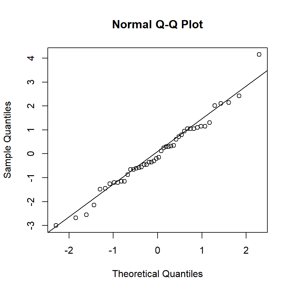
Figure 9.6: Quantile-quantile plot of residuals.
Figure 9.6 indicates that the residuals lie roughly on a straight line. To formally check, we can undertake a Shapiro-Wilk test. The null hypothesis for this test is that the data come from a normally distributed population.
shapiro.test(plant.aov$residuals)
    Shapiro-Wilk normality test

data:  plant.aov$residuals
W = 0.98038, p-value = 0.6216
We see from the results that the \(p\)-value is large (0.62), thus, there is no evidence to reject the null hypothesis and we can conclude that the data are normally distributed.
All the assumptions have been checked (as far as possible) and are valid for these plant data. Thus, we can move on with the analysis to determine where differences lie.
9.4 Identifying differences (and more on multiple comparisons)
ANOVA identifies whether, or not, a difference exists between at least one pair of group means. If a difference exists, the next stage is to identify which pairs of groups are different and how large any differences might be. There will be three pairwise comparisons for three groups (B-N, B-P and N-P) but the number soon increases with more groups; the number is given by for \(k\) groups:
\[\textrm{number of pairwise comparisons} = \frac{k!}{(k-2)!2!}\]
We could build 95% confidence intervals for each pairwise comparison but each has a Type I error rate of 5%; these errors compound and so we can adjust the error rate so that the overall, or family wise, error rate is 5%. There are various methods of making this adjustment and here we look at two methods (Bonferroni and Sidak corrections) and Tukey’s Honest Significance Differences for adjusted confidence intervals.
Q9.2 If there are four groups to be compared (as in Q9.1), how many pairwise comparisons can be made?
9.4.1 Sidak correction
Let the probability of a Type I error be \(\alpha_1\). Hence, the probability of not making a Type I error is given by \(1 - \alpha_1\) and so the probability of not making a Type I error for a series of \(c\) tests is \((1 - \alpha_1)^c\), assuming that the tests are independent. Thus, the probability of making an error with the series of tests is \(1 - (1 - \alpha_1)^c\). We would like this probability to equal \(\alpha\) and rearranging this equation provides the Sidak correction.
The Sidak correction for the new threshold \(p\)-value is calculated from:
\[\alpha_{adj} = 1 - (1-\alpha)^{\frac{1}{c}}\]
where
- \(\alpha_{adj}\) is the new threshold,
- \(\alpha\) is the desired Type I error collectively (family error rate) and
- \(c\) is the number of comparisons.
Example We have a control treatment and plan to compare it against 3 different treatments (so \(c\)=3) and require an overall Type I error of 5%:
\[\alpha_{adj} = 1 - (1 - 0.05)^{\frac{1}{3}}=0.01695\]
Rather than accept a result as significant if the probability is below 0.05, we accept it as significant if the \(p\)-value for each test is below 0.01695.
9.4.2 Bonferroni correction
A simpler method (and therefore more well-known) is the Bonferroni correction; we calculate a new threshold \(p\)-value by dividing the desired Type I error rate (overall comparisons), by the number of comparisons:
\[\alpha_{adj} = \frac{\alpha}{c}\]
Example We want to conduct a series of 5 two sample \(t\) tests with a desired overall error rate of 5%. The adjusted error rate is thus, \(\alpha_{adj} = 0.05/5 = 0.01\). Therefore, a \(p\)-value < 0.01 is required to conclude a significant result for each comparison.
This method is considered to be ‘conservative’ with respect to the family wise error rate, particularly if there are a large number of tests, or comparisons. This correction comes at the cost of increasing the Type II error.
Q9.3 We would like to make a series of 6 comparisons with an overall, family wise error rate of 0.05. What will the adjusted error rate be for each test using both the Sidak and Bonferroni corrections? Which correction is more stringent?
9.4.3 Tukey’s Honest Significant Difference (HSD)
This method is similar to creating confidence intervals for differences between two means but modifies the standard error and multiplier resulting in wider confidence intervals. We then check to see if zero is contained within each CI to determine whether any pair of group means are significantly different with a family wise error rate of \(\alpha\).
Example We return to the data of titanium levels in plants grown in three different types of growing medium; previously we found that a difference does exist. We calculate Tukey’s HSD for the pairwise comparisons to decide where any differences might lie (Table 9.5).
| diff | lwr | upr | p adj | |
|---|---|---|---|---|
| N-B | 2.478 | 0.9545 | 4.001 | 0.0008236 |
| P-B | 3.75 | 2.54 | 4.96 | 6.734e-09 |
| P-N | 1.272 | -0.1009 | 2.645 | 0.07432 |
the first column indicates the two groups being compared,
‘diff’ is the point estimate of the difference in means between the two groups,
‘lwr’ and ‘upr’ are the lower and upper bounds, respectively, of the confidence interval for the difference taking into account the multiple comparisons, and
‘\(p\) adj’ is the \(p\)-value evaluating the null hypothesis that the difference between the means of the populations is zero taking into account the number of multiple comparisons.
In this case, one confidence interval contains zero (i.e. P-N); on average the mean titanium level in group P is between -0.1 units lower to 2.65 units higher than group N. An interval containing zero indicates that zero is a plausible value for the difference in means, thus the means for these two groups are not significantly different.
The other intervals are significantly different - the interval does not contain zero. The mean titanium level in N is significantly higher than B - on average 0.95 to 4.00 units higher (95% confidence). Also, the level in P is significantly higher than in B - on average 2.54 to 4.96 units higher (95% confidence)
As a comparison, Table 9.6 shows that standard 95% confidence intervals for each of the difference in means are slightly narrower than the confidence intervals obtained using Tukey’s HSD (Table 9.5).
| Group | lwr | upr |
|---|---|---|
| N-B | 1.086 | 3.87 |
| P-B | 2.785 | 4.715 |
| P-N | -0.05809 | 2.603 |
9.4.3.1 Doing this in R
# Create ANOVA object
plant.aov <- aov(Ti ~ Group, data=plant)
# Tukeys HSD
TukeyHSD(plant.aov)
Tukey multiple comparisons of means
95% family-wise confidence level
Fit: aov(formula = Ti ~ Group, data = plant)
$Group
diff lwr upr p adj
N-B 2.477778 0.9544691 4.001086 0.0008236
P-B 3.750000 2.5402571 4.959743 0.0000000
P-N 1.272222 -0.1008697 2.645314 0.0743237These intervals can be displayed with a helpful dashed line allowing confidence intervals containing zero to be easily identified:
# Plot Tukeys HSD
plot(TukeyHSD(plant.aov))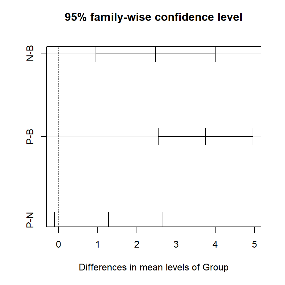
Figure 9.7: Comparison of titanium levels in groups B, N and P. The horizontal black lines indicate Tukey’s HSD confidence interval for the pairwise comparison. The dashed line means it is easy to identify CI that include zero.
Q9.4 The following are Tukey’s HSD comparing the petrol prices for four different locations.
TukeyHSD(aov(prices ~ location, data=petrol)) Tukey multiple comparisons of means
95% family-wise confidence level
Fit: aov(formula = prices ~ location, data = petrol)
$location
diff lwr upr p adj
Motorway-City 8.201950 1.191987 15.2119125 0.0164806
Rural-City 5.075935 -1.934027 12.0858982 0.2258147
Town-City -2.408140 -9.418102 4.6018231 0.7915806
Rural-Motorway -3.126014 -10.135977 3.8839485 0.6301923
Town-Motorway -10.610089 -17.620052 -3.6001266 0.0013224
Town-Rural -7.484075 -14.494038 -0.4741123 0.0326058a. Which locations are significantly different and which are not, testing at a significance level of 5%?
b. Which two locations have the largest difference in means?
9.4.4 Multiple comparison dilema
In making adjustments when performing multiple comparisons, we are trading one error for another; we control a Type I error at the cost of a Type II error. For example, when making multiple comparisons, the adjustments reduce the threshold probability level used to determine significance. This means that we won’t make many Type I errors, but Type II errors could be large. This relates to a concept called power, which is covered in chapter 10.
The choice of whether, or not, to make any adjustment is not straightforward and is generally context specific:
- sometimes people think adjustments should be made because they are really worried about Type I errors/false positives (e.g. concluding a treatment is effective when it isn’t)
- sometimes making a Type II error/false negative could be concerning (e.g. when exploring new cancer drugs a promising drug might be missed).
9.5 Two-way ANOVA
So far we have compared data where there has been only one division of the data into groups (e.g. growing medium) and so specifically we have considered one-way ANOVA. Frequently, we may need to account for an additional discrete variable (e.g. plant variety). This can be done using a two-way ANOVA.
Like many statistical methods, ANOVA arose out of research in agricultural science and so the terminology used frequently references its development and here we use an agricultural example to illustrate its use (after (ClarkeCooke1998?).
Suppose we are interested in the crop yield of 5 different varieties of a plant (e.g. potato). A large field is divided into 20 (4 by 5) small units (or plots) and each variety (denoted by A to E) is randomly assigned to 4 plots (Table @ref(tab:crd.example)). All plants are cultivated in the same way and each plot receives the same amount of fertilizer, for example. Thus, the only reason for systematic variation between plots would be different varieties. This design, where varieties were assigned to plots completely at random is known as a completely randomised design. We could analyse the data arising from this experiment with a one-way ANOVA.
| C | D | A | C | B |
| B | B | D | E | E |
| C | A | B | C | D |
| A | D | A | E | E |
It may be that there are differences within the field (e.g. fertility, drainage, depth of soil) such that even if the same variety was planted, the crop yield would differ in different parts of the field. Thus, when comparing the different varieties we also need to account for the differences in the field. To account for these differences, the field is divided into blocks (based on fertility, for example); each block contains enough plots to accommodate each variety once. In this example, a block would consist of 5 plots and each variety is randomly assigned to plots in each block (Table @ref(tab:rbd.example)). This is known as a randomised block design. The analysis is by a two-way ANOVA to account for differences between blocks and varieties.
| E | D | C | B | A |
| E | C | A | B | D |
| D | C | A | B | E |
| D | A | B | C | E |
9.5.1 Calculating a two-way ANOVA table
To calculate a two-way ANOVA table, we extend the one-way table (Table 9.7).
| Source of variation | df | Sum Sq | Mean Sq | \(F\) value |
|---|---|---|---|---|
| Between groups | \(k-1\) | \(SS_G\) | \(s_G^2\) | \(f_0\) |
| Between blocks | \(b-1\) | \(SS_B\) | \(s_B^2\) | \(f_B\) |
| Residuals | \((k-1)(b-1)\) | \(SS_W\) | \(s_W^2\) | |
| ————— | ————– | ——— | ———- | – |
| Total | \(n_{tot}-1\) |
where:
\(s_B^2\) is the mean sum of squares between blocks and
\[s_B^2 = \frac{SS_B}{b-1}\]
We don’t provide all formulae here for calculating the components of the ANOVA table and note some formula have changed compared to a one-way ANOVA (e.g. \(SS_W\)) but we illustrate the table with an example below. However, as before, the test statistic for testing the null hypothesis that all groups means are the same is given by:
\[f_0 = \frac{s_G^2}{s_W^2}\]
We can also test the null hypothesis that the block means are the same:
\[f_B = \frac{s_B^2}{s_W^2}\]
Example Let’s return to the study looking at the mean titanium levels in plants grown in different growing mediums. Suppose that the plants were exposed to different light levels (classified as low, medium and high) and we want to take this into account in a two-way ANOVA.
# Fit two-way ANOVA
plant.aov <- aov(Ti ~ Group + Light, data=plant)
# Display ANOVA table
summary(plant.aov)
Df Sum Sq Mean Sq F value Pr(>F)
Group 2 118.60 59.30 27.369 2.82e-08 ***
Light 2 1.22 0.61 0.283 0.755
Residuals 41 88.83 2.17
---
Signif. codes: 0 '***' 0.001 '**' 0.01 '*' 0.05 '.' 0.1 ' ' 1As before, there are significant differences in the mean titanium levels between different growing mediums.
The formulae to calculate test statistic for blocks follows the same pattern as for a one-way ANOVA:
\[s_B^2 = \frac{SS_B}{b-1} = \frac{1.22}{2} = 0.61\]
\[f_B = \frac{s_B^2}{s_W^2} = \frac{0.61}{2.17} = 0.28\]
The reference distribution is \(F_{df1=b-1, df2=(k-1)(b-1)}\):
# p=value for blocks
pf(0.283, df1=2, df2=41, lower.tail=FALSE)
[1] 0.7549797The \(p\)-value is large and so the null hypothesis for blocks cannot be rejected in this example.
9.6 Alternative tests to ANOVA
If the data do not fulfill the test assumptions of normality and constant spread (or equal standard deviations), alternative tests are available and two are briefly described below. Although some assumptions can be relaxed with these tests, other assumptions can not.
If the data are not normally distributed, the Kruskal-Wallis test can be used as a non-parametric alternative to ANOVA; it can be thought of as a multi-level version of the Mann-Whitney test (chapter 8). However, this test does still assume that the groups have the same standard deviation. This test uses ranks and the null hypothesis is that the mean ranks of the groups is the same. The test statistic follows a \(\chi^2\) (chi-square) distribution which is indexed by one parameter, the degrees of freedom; this distribution is discussed in chapter 12.
If the groups do not have similar standard deviations (heteroscedastic), an adaptation to ANOVA, called Welch’s ANOVA, can be used, although this still requires that the data are normally distributed.
9.6.1 Doing this in R
The Kruskal-Wallis test is performed with the kruskal.test function:
kruskal.test(Ti ~ Group, data=plant)
    Kruskal-Wallis rank sum test

data:  Ti by Group
Kruskal-Wallis chi-squared = 26.286, df = 2, p-value = 1.959e-06
The \(p\)-value is interpreted in the same way; here it is very small, providing evidence to reject the null hypothesis. There is also a function which provides multiple comparisons after the Kruskal-Wallis test (Siegel and Castellan 1988); this requires the pgirmess library (Giraudoux 2021). It identifies differences between groups depending on the specified significance level (0.05 by default).
library(pgirmess)
kruskalmc(Ti ~ Group, data=plant)
Multiple comparison test after Kruskal-Wallis
p.value: 0.05
Comparisons
obs.dif critical.dif difference
B-N 15.085470 13.93401 TRUE
B-P 23.682692 11.06576 TRUE
N-P 8.597222 12.55995 FALSEWelch’s ANOVA is performed using welch.test which is in the onewaytests library (Dag et al. 2021) (this is not part of the base libraries and so will need to be installed). Again it gives helpful output.
library(onewaytests)
welch.test(Ti ~ Group, data=plant)
  Welch's Heteroscedastic F Test (alpha = 0.05)
-------------------------------------------------------------
  data : Ti and Group

  statistic  : 30.83309
  num df     : 2
  denom df   : 19.47308
  p.value    : 9.232681e-07

  Result     : Difference is statistically significant.
-------------------------------------------------------------
9.7 Summary
Analysis of variance, the procedure for comparing differences in means for more than two groups is a frequently used procedure. Technically we have described a one-way ANOVA because data are divided by only one factor, i.e. the different groups. Two-way ANOVA is used where two factors are be taken into account. As with any statistical test, there are underlying assumptions which need to be met for the results to be valid and an appropriate test needs to be selected based on the data.
The significance level (\(\alpha\)) is the probability of rejecting the null hypothesis when it is true (Type I error) and we want this to be small. The level should be set prior to any test and is the level you are happy to reject the null hypothesis. A value of \(\alpha=0.05\) is frequently used but to decrease the chance of making a Type I error, a value of \(\alpha=0.01\) is sometimes used.
Most of the R functions provide an exact \(p\)-value associated with the test statistic - this is the probability of obtaining the test statistic, and one more extreme, if the null hypothesis is true. It is found from the area under the reference distribution associated with the test statistic. To decide whether to reject the null hypothesis, the \(p\)-value is compared to the \(\alpha\) level set prior to the test. A \(p\)-value less than \(\alpha\) provides evidence to reject the null hypothesis and a \(p\)-value greater than \(\alpha\) does not provide evidence to reject the null hypothesis.
If statistically significant differences are detected, then we want to determine where the differences lie. Comparing multiple pairwise combinations of groups increases the risk of making a Type I error and so to ensure that the desired error rate applies over all comparisons an adjustment can be made.
In this chapter we have concentrated on the Type I error for a test; the Type II error is considered in a later chapter.
More information about the \(F\) test for ANOVA can be found here
9.7.1 Learning outcomes
In this chapter we have:
undertaken a one-way analysis of variance to determine differences between more than two groups,
determined where differences between groups lie,
checked the test assumptions, and
if the assumptions for ANOVA are not fulfilled, seen that an alternative test can be used.
9.8 Answers
Q9.1 a. The null hypothesis is that the mean petrol price is the same in all four locations:
\[H_0: \mu_{City} = \mu_{Motorway} = \mu_{Rural} = \mu_{Town} \] The alternative hypothesis is that at least one location has a different mean petrol price to one other location.
Q9.1 b. The completed ANOVA table is given below and the \(F\) test statistic is 6.77.
| Source of variation | df | Sum Sq | Mean Sq | \(F\) value |
|---|---|---|---|---|
| Between locations | 3 | 668.4 | 229.47 | 6.77 |
| Residuals | 36 | 1220.47 | 33.90 | |
| —————— | ————– | ——— | ———- | – |
| Total | 39 |
Each component of the table is calculated as follows where \(k = 4\) groups.
\[\begin{equation}\label{} \begin{split} SS_B & = \sum_{i=1}^{k} n_i (\bar{x}_{i.}-\bar{x}_{..})^2 \\ & = 10(135.4 - 138.1)^2 + 10(143.6 - 138.1)^2 + 10(140.4 - 138.1)^2 + 10(133.0 - 138.1)^2\\ & = 688.4 \end{split} \end{equation}\]
\[s^2_B = \frac{SS_B}{k-1} = \frac{688.4}{4-1} = 229.47\]
\[\begin{equation} \begin{split} SS_W & = \sum_{i=1}^{k}(n_i-1)s_i^2 \\ & = (10-1)5.52^2 + (10-1)3.84^2 + (10-1)6.43^2 + (10-1)7.00^2\\ & = 1220.47 \end{split} \end{equation}\]
\[s^2_W = \frac{SS_W}{n_{tot}-k} = \frac{1220.47}{40 - 4} = 33.90\] Finally,
\[f_0 = \frac{s^2_B}{s^2_W} = \frac{229.47}{33.90} = 6.77\]
Q9.1 c. The critical value is 2.866 which is smaller than the \(F\) test statistic. Hence, there is evidence to reject the null hypothesis and conclude that at least one location has a different mean petrol prices to one other location.
Q9.2 If there are four groups, there will be 6 possible pairwise comparisons (see Q9.4).
Q9.3 The adjusted error rates are:
Sidak correction \[1 - (1 - 0.05)^{\frac{1}{6}} = 0.0085\]
Bonferroni correction: \[\frac{0.05}{4} = 0.0083\]
The Bonferroni correction will be the more stringent (requiring a higher level of evidence) because the adjusted significance level is smaller than the Sidak correction.
Q9.4 a. The locations which are significantly different are Motorway-City, Town-Motorway and Town-Rural; these CI have a small \(p\)-value (<0.05) and do not contain zero. The locations which are not significantly different are Rural-City, Town-City and Rural-Motorway.
Q9.4 b. The largest difference is between Town and Motorway. On average, the price in Town is 3.6 to 17.6 pence per litre lower than the price in the Motorway.