Post Impact Changes

Load data

count.data <- readRDS("data/nystedphaseA.rds")
panelid <- as.numeric(count.data$TransectID)
nysted.bndwf <- nysted.bndwf/1000
nysted.studybnd <- nysted.studybnd/1000

initialModel<-MRSea::gamMRSea(Count ~ 1 + as.factor(YearMonth)+Depth +
                      x.pos + y.pos + offset(log(Area)),  data=count.data,
                      family=quasipoisson)

Site wide effect

First we will generate a site-wide change of a 40% decline in abundance. This means that we want 60% of the current population and this is the pct.change parameter.

Here we assume that the post impact survey regime is the same as pre impact. This can be altered for the power analysis to increase or decrease the number of surveys.

# generate a 20% site-wide change:
changedata.oc <-genChangeData(pct.change=60, 
                           model=initialModel, 
                           data=count.data,
                           panels = "TransectID")

As a sense check, it is wise to summarise our generated data pre and post change to ensure our desired increase/decrease has been observed (in this case a 20% decline in average numbers). We can also check at this point that we have equal numbers of observations before and post event.

require(dplyr)
t<-group_by(changedata.oc, eventphase)%>%
  summarise(sum=sum(truth), mean=mean(truth), n=n())
t

 [38;5;246m# A tibble: 2 × 4 [39m
  eventphase    sum  mean     n
        [3m [38;5;246m<dbl> [39m [23m   [3m [38;5;246m<dbl> [39m [23m  [3m [38;5;246m<dbl> [39m [23m  [3m [38;5;246m<int> [39m [23m
 [38;5;250m1 [39m          0  [4m2 [24m [4m6 [24m714.  4.11   [4m6 [24m500
 [38;5;250m2 [39m          1  [4m1 [24m [4m6 [24m028.  2.47   [4m6 [24m500

Rasterise the before and after data:

rdf1<-make.raster(ncell.y=50, 
                  xyzdata=changedata.oc %>% filter(eventphase==0) %>%
                    dplyr::select("x.pos", "y.pos", "truth"), 
                  z.name = "Mean.count")

rdf2<-make.raster(ncell.y=50, 
                  xyzdata=filter(changedata.oc, eventphase==1) %>%
                    dplyr::select("x.pos", "y.pos", "truth"),
                  z.name="Mean.count")

rdf<-rbind(data.frame(rdf1, evph=0), data.frame(rdf2, evph=1))

Find the percentage change in each grid cell (you could do this for absolute difference if you prefer)

pct.change<-((rdf$Mean.count[rdf$evph==1] - rdf$Mean.count[rdf$evph==0])/
               rdf$Mean.count[rdf$evph==0])*100

Plot the data

ggplot( NULL ) + geom_raster( data = rdf1 , aes( x , y , fill = pct.change ) ) +
  scale_fill_gradientn(colours=mypalette,values=c(0,1), space = "Lab", 
                       na.value = "grey50", guide = "colourbar") + 
  theme_bw() + coord_equal() +
  geom_path(data = nysted.bndwf, aes(x.pos, y.pos)) +
  geom_path(data = nysted.studybnd, aes(x.pos, y.pos))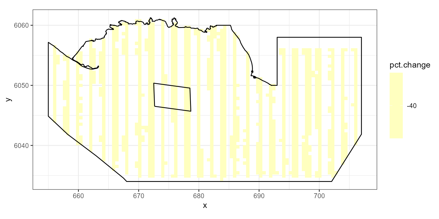

ggplot() +
  geom_raster(data = rdf , aes(x , y , fill = Mean.count)) +
  facet_wrap(~evph) +
  coord_equal() + theme_bw() +
  scale_fill_distiller(palette = "Spectral",name="Animal Counts") +
  geom_path(data = nysted.bndwf, aes(x.pos, y.pos)) +
  geom_path(data = nysted.studybnd, aes(x.pos, y.pos))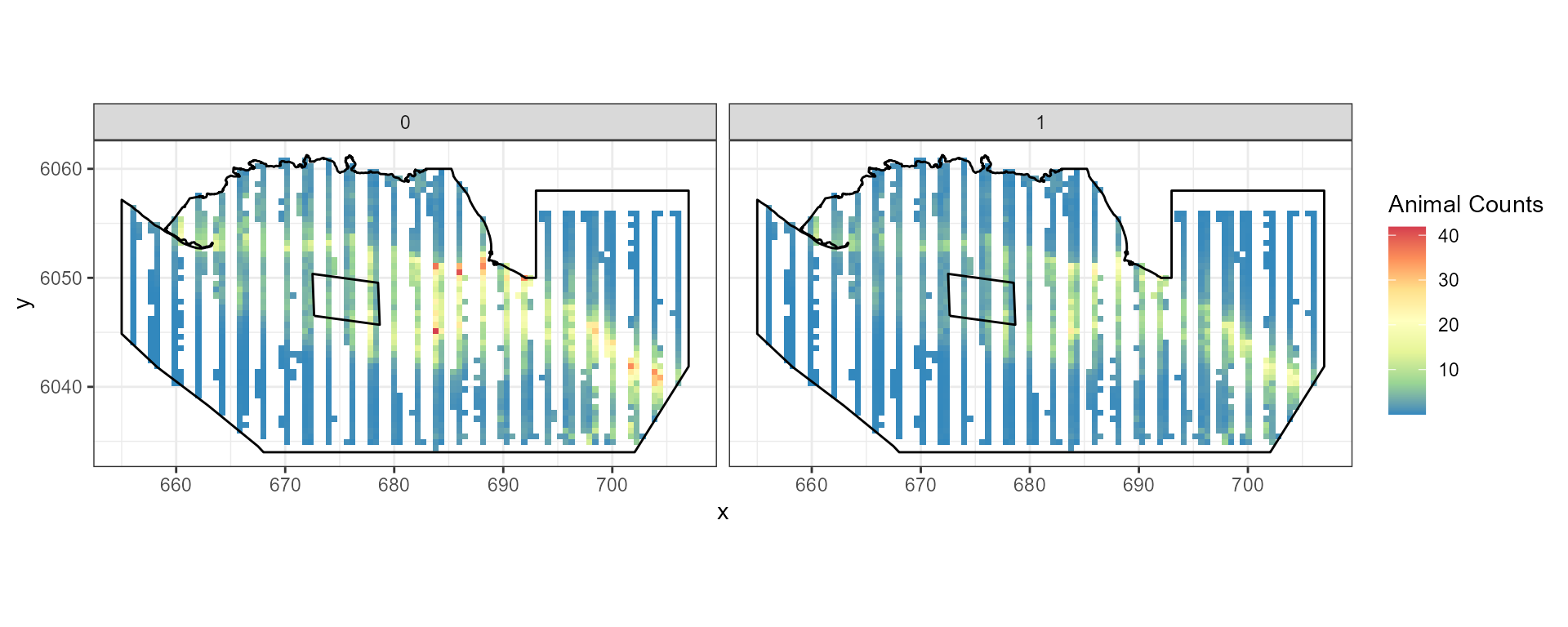

Redistribution

To maintain the same number of animals in the study area but generate a decline in and around the footprint with re-distribution elsewhere we use the pct.change parameter to specify the decline and the eventsite.bnd parameter to specify the region for that decline.

# generate a 50% decline in the windfarm footprint:

ggplot() + 
  geom_point(data = count.data, aes(x.pos, y.pos), colour = "grey") +
  theme_bw() + 
  geom_path(data = nysted.bndwf, aes(x.pos, y.pos))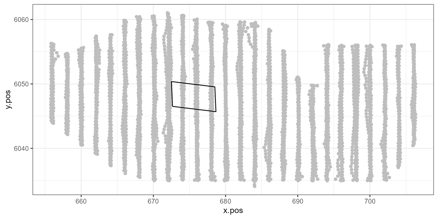

changedata.re<-genChangeData(pct.change=60,
                            eventsite.bnd=nysted.bndwf, 
                            model=initialModel, 
                            data=count.data, 
                            panels="TransectID")

require(dplyr)
t<-group_by(changedata.re, eventphase)%>%
  summarise(sum=sum(truth), mean=mean(truth), n=n())
t

 [38;5;246m# A tibble: 2 × 4 [39m
  eventphase    sum  mean     n
        [3m [38;5;246m<dbl> [39m [23m   [3m [38;5;246m<dbl> [39m [23m  [3m [38;5;246m<dbl> [39m [23m  [3m [38;5;246m<int> [39m [23m
 [38;5;250m1 [39m          0  [4m2 [24m [4m6 [24m714.  4.11   [4m6 [24m500
 [38;5;250m2 [39m          1  [4m2 [24m [4m6 [24m714.  4.11   [4m6 [24m500

Rasterise the before and after data:

rdf1.re<-make.raster(ncell.y=30, 
                  xyzdata=changedata.re %>% filter(eventphase==0) %>%
                    dplyr::select("x.pos", "y.pos", "truth"), 
                  z.name = "Mean.count")

rdf2.re<-make.raster(ncell.y=30, 
                  xyzdata=filter(changedata.re, eventphase==1) %>%
                    dplyr::select("x.pos", "y.pos", "truth"),
                  z.name="Mean.count")

rdf.re<-rbind(data.frame(rdf1.re, evph=0), data.frame(rdf2.re, evph=1))

Find the percentage change in each grid cell (you could do this for absolute difference if you prefer)

pct.change.re<-((rdf.re$Mean.count[rdf.re$evph==1] - rdf.re$Mean.count[rdf.re$evph==0])/
               rdf.re$Mean.count[rdf.re$evph==0])*100

Plot the data

ggplot( NULL ) + geom_raster( data = rdf1.re , aes( x , y , fill = pct.change.re ) ) +
  scale_fill_gradientn(colours=mypalette,values=c(0,1), space = "Lab", 
                       na.value = "grey50", guide = "colourbar") + 
  theme_bw() + coord_equal() +
  geom_path(data = nysted.bndwf, aes(x.pos, y.pos)) +
  geom_path(data = nysted.studybnd, aes(x.pos, y.pos))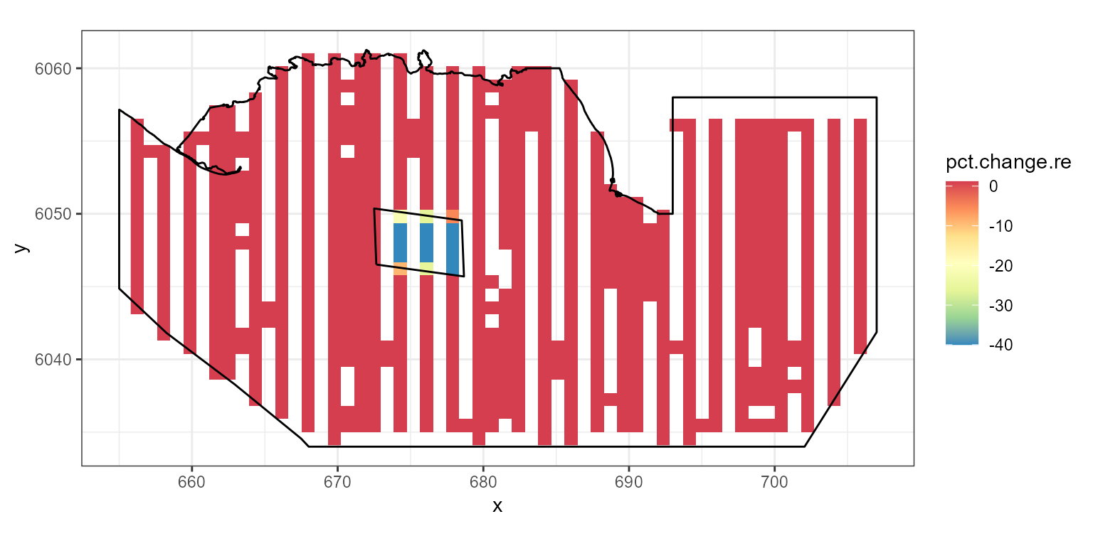

ggplot() +
  geom_raster(data = rdf.re , aes(x , y , fill = Mean.count)) +
  facet_wrap(~evph) +
  coord_equal() + theme_bw() +
  scale_fill_distiller(palette = "Spectral",name="Animal Counts")+
  geom_path(data = nysted.bndwf, aes(x.pos, y.pos)) +
  geom_path(data = nysted.studybnd, aes(x.pos, y.pos))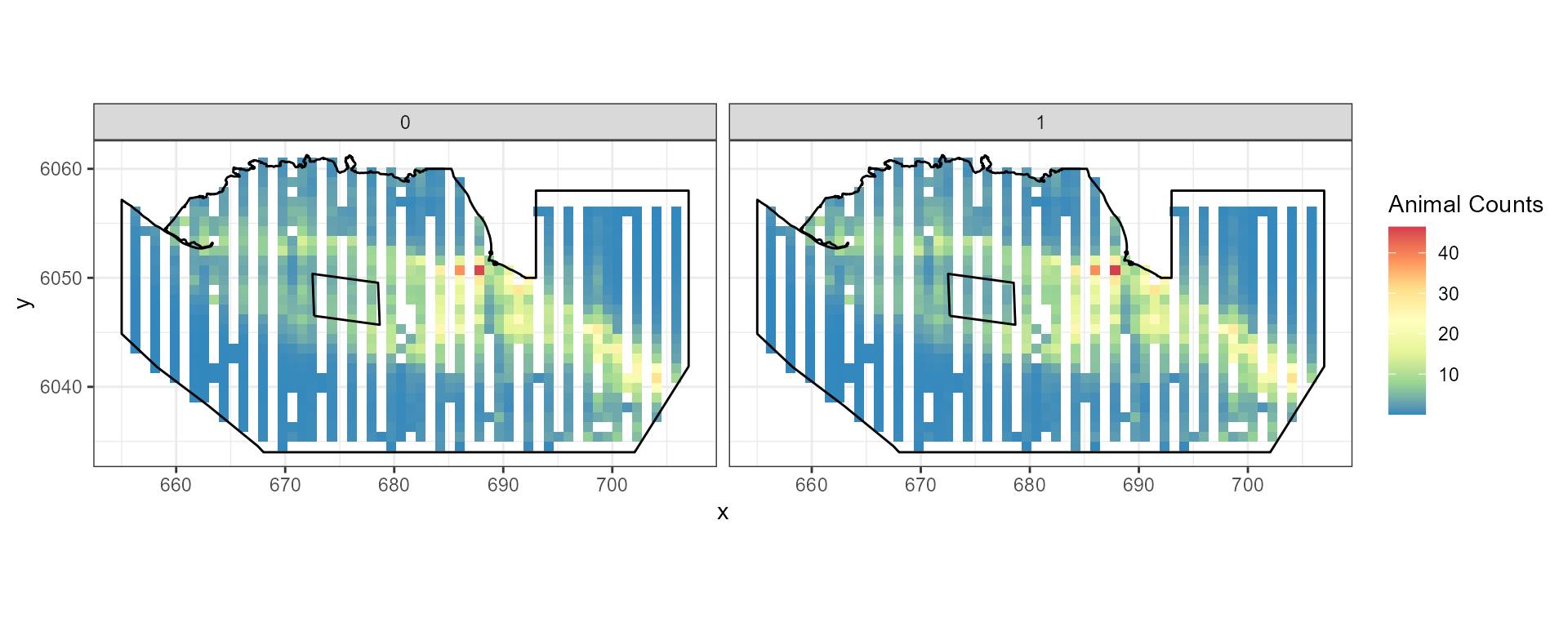

Redistribution and Site Wide

Combining an overall change and a redistribution needs two parameters for pct.change. The first is the redistribution and the second the overall change. Here we show a decline in the footprint of 40%, with redistribution and an overall change of 10%.

# generate a 50% decline in the windfarm footprint:
changedata.ocre<-genChangeData(pct.change=c(60, 90),
                            eventsite.bnd=nysted.bndwf, 
                            model=initialModel, 
                            data=count.data, 
                            panels="TransectID")

require(dplyr)
t<-group_by(changedata.ocre, eventphase)%>%
  summarise(sum=sum(truth), mean=mean(truth), n=n())
t

 [38;5;246m# A tibble: 2 × 4 [39m
  eventphase    sum  mean     n
        [3m [38;5;246m<dbl> [39m [23m   [3m [38;5;246m<dbl> [39m [23m  [3m [38;5;246m<dbl> [39m [23m  [3m [38;5;246m<int> [39m [23m
 [38;5;250m1 [39m          0  [4m2 [24m [4m6 [24m714.  4.11   [4m6 [24m500
 [38;5;250m2 [39m          1  [4m2 [24m [4m4 [24m043.  3.70   [4m6 [24m500

Rasterise the before and after data:

rdf1.ocre<-make.raster(ncell.y=30, 
                  xyzdata=changedata.ocre %>% filter(eventphase==0) %>%
                    dplyr::select("x.pos", "y.pos", "truth"), 
                  z.name = "Mean.count")

rdf2.ocre<-make.raster(ncell.y=30, 
                  xyzdata=filter(changedata.ocre, eventphase==1) %>%
                    dplyr::select("x.pos", "y.pos", "truth"),
                  z.name="Mean.count")

rdf.ocre<-rbind(data.frame(rdf1.ocre, evph=0), data.frame(rdf2.ocre, evph=1))

Find the percentage change in each grid cell (you could do this for absolute difference if you prefer)

pct.change.ocre<-((rdf.ocre$Mean.count[rdf.ocre$evph==1] - rdf.ocre$Mean.count[rdf.ocre$evph==0])/
               rdf.ocre$Mean.count[rdf.ocre$evph==0])*100

Plot the data

ggplot( NULL ) + geom_raster( data = rdf1.ocre , aes( x , y , fill = pct.change.ocre) ) +
  scale_fill_gradientn(colours=mypalette,values=c(0,1), space = "Lab", 
                       na.value = "grey50", guide = "colourbar") + 
  theme_bw() + coord_equal() +
  geom_path(data = nysted.bndwf, aes(x.pos, y.pos)) +
  geom_path(data = nysted.studybnd, aes(x.pos, y.pos))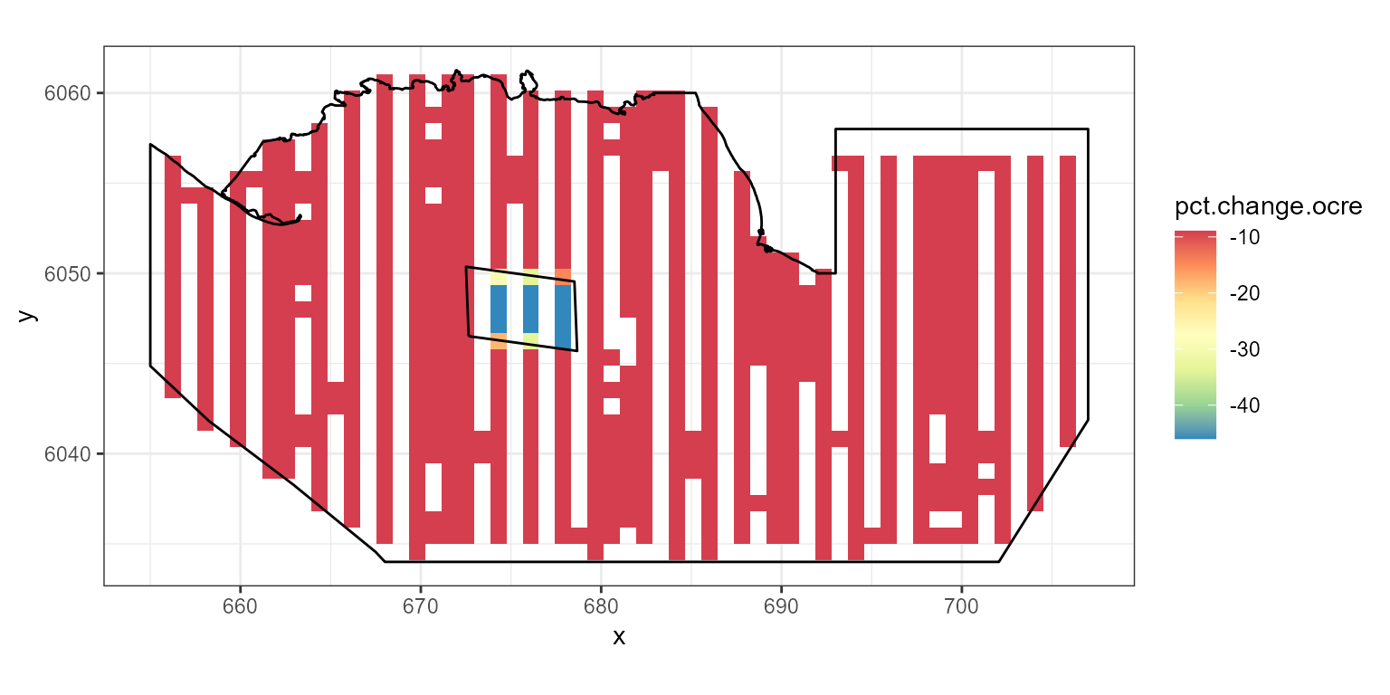

ggplot() +
  geom_raster(data = rdf.ocre, aes(x , y , fill = Mean.count)) +
  facet_wrap(~evph) +
  coord_equal() + theme_bw() + 
  scale_fill_distiller(palette = "Spectral",name="Animal Counts")+
  geom_path(data = nysted.bndwf, aes(x.pos, y.pos)) +
  geom_path(data = nysted.studybnd, aes(x.pos, y.pos))

LAS Scott-Hayward

2025-03-20

Site wide effect

Redistribution

Redistribution and Site Wide