Using the Tweedie Distribution

This document shows how to fit a gamMRSea model using the Tweedie distribution.

The Tweedie distribution

The variance of the Tweedie distribution is parametrised by the mean $\mu$ and the dispersion parameter $\phi$ :

$Var(y) = V(\mu)\phi = \mu^\xi\phi$

The following distributions can be achieved by specifying the following values for $\xi$

Gaussian ( $\xi = 0$ )
Poisson ( $\xi = 1$ )
Gamma ( $\xi = 2$ )
Inverse Gaussian ( $\xi = 3$ )

For zero inflated data, i.e. the response distribution has mass at zero (i.e., it has exact zeros) but is otherwise continuous on the positive real numbers, the values of $\xi$ between 1 and 2 are particularly useful to us.

An example of fitting the tweedie distribution in `R`

library(statmod)
glm(y ~ x, data=data, 
    family=tweedie(var.power = 1.1, link.power=0))

In this example, $\xi = 1.1$ and the model can be described as:

$y_i \sim Tw(\mu_{i}, \phi, \xi)$

where $log(\mu_i) = \beta_0 + \beta_1x_i$

and $Var(y_i) = \mu_i^{1.1} \phi$

var.power specifies the value for $\xi$ and link.power = 0 indicates a log link is used.

For example, tweedie(var.power=1, link.power=0) is equivalent to quasipoisson(link="log"). Note: it is not equivalent to poisson(link="log") as the dispersion is not set equal to 1.

Setup

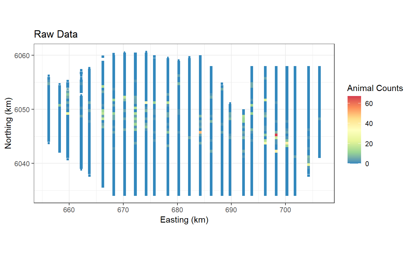
Load some data
Fit a simple intercept only model and show the link between tweedie and quasipoisson.

library(MRSea)
library(dplyr)
library(ggplot2)

# load data
data(ns.data.re)

Two additional libraries are required for model fitting and selection. statmod provides the model family tweedie() and the tweedie package contains an appropriate AIC.

library(statmod)
library(tweedie)

Fit a Tweedie model with $\xi = 1$ and a log link function.

fit_tw<- glm(birds ~ 1, family=tweedie(var.power=1, link.power = 0),data=ns.data.re)
summary(fit_tw)
#> 
#> Call:
#> glm(formula = birds ~ 1, family = tweedie(var.power = 1, link.power = 0), 
#>     data = ns.data.re)
#> 
#> Deviance Residuals: 
#>    Min      1Q  Median      3Q     Max  
#> -1.717  -1.717  -1.717  -1.717  37.696  
#> 
#> Coefficients:
#>             Estimate Std. Error t value Pr(>|t|)    
#> (Intercept)  0.38773    0.02399   16.16   <2e-16 ***
#> ---
#> Signif. codes:  0 '***' 0.001 '**' 0.01 '*' 0.05 '.' 0.1 ' ' 1
#> 
#> (Dispersion parameter for Tweedie family taken to be 23.56597)
#> 
#>     Null deviance: 186644  on 27797  degrees of freedom
#> Residual deviance: 186644  on 27797  degrees of freedom
#> AIC: NA
#> 
#> Number of Fisher Scoring iterations: 7

Fit the equivalent model using the quasipoisson distribution.

fit_qp<- glm(birds ~ 1, family=quasipoisson(link="log"),data=ns.data.re)
summary(fit_qp)
#> 
#> Call:
#> glm(formula = birds ~ 1, family = quasipoisson(link = "log"), 
#>     data = ns.data.re)
#> 
#> Deviance Residuals: 
#>    Min      1Q  Median      3Q     Max  
#> -1.717  -1.717  -1.717  -1.717  37.696  
#> 
#> Coefficients:
#>             Estimate Std. Error t value Pr(>|t|)    
#> (Intercept)  0.38773    0.02399   16.16   <2e-16 ***
#> ---
#> Signif. codes:  0 '***' 0.001 '**' 0.01 '*' 0.05 '.' 0.1 ' ' 1
#> 
#> (Dispersion parameter for quasipoisson family taken to be 23.56596)
#> 
#>     Null deviance: 186644  on 27797  degrees of freedom
#> Residual deviance: 186644  on 27797  degrees of freedom
#> AIC: NA
#> 
#> Number of Fisher Scoring iterations: 7

Note that the two model outputs are identical. In reality though we need to find out what value of $\xi$ is best for our data. For this we can use the tweedie.profile function from the tweedie library.

Note: this function can take a long time to run.

profout <- tweedie.profile(birds ~ 1, 
                           data=ns.data.re,
                           xi.vec = seq(1.01, 1.99, by=0.05), do.plot=TRUE)
#> 1.01 1.06 1.11 1.16 1.21 1.26 1.31 1.36 1.41 1.46 1.51 1.56 1.61 1.66 1.71 1.76 1.81 1.86 1.91 1.96 
#> ....................Done.

profout2 <- tweedie.profile(birds ~ MonthOfYear + x.pos + y.pos + Year, 
                           data=ns.data.re,
                           xi.vec = seq(1.01, 1.99, by=0.05), do.plot=TRUE)
#> 1.01 1.06 1.11 1.16 1.21 1.26 1.31 1.36 1.41 1.46 1.51 1.56 1.61 1.66 1.71 1.76 1.81 1.86 1.91 1.96 
#> ....................Done.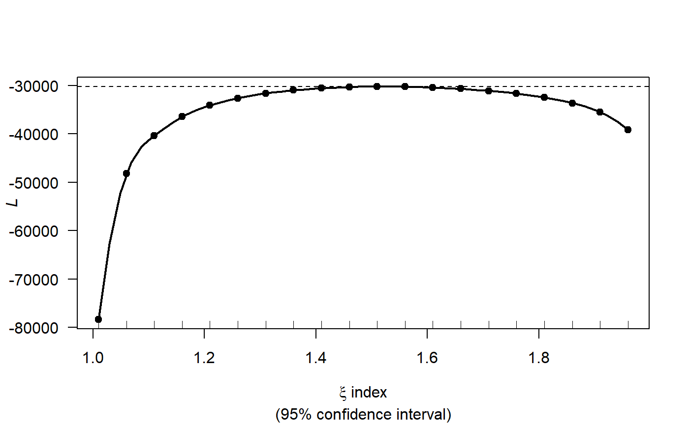

profout$xi.max
#> [1] 1.533469
profout2$xi.max
#> [1] 1.514082

Fitting a `gamMRSea` model

Lets fit a model to the data using one smooth variable; month of the year.

varlist=c('x.pos')
ns.data.re$response <- ns.data.re$birds

Set up the initial model with the Tweedie distribution parameterised with the log link function (link.power=0) and the variance power ( $\xi$ ) equal to our output from the profiling (var.power =).

initialModel<- glm(response ~ 1, family=tweedie(var.power=profout2$xi.max, link.power = 0),data=ns.data.re)

Remember to specify a Tweedie specific fitness measure of either AICtweedie or BICtweedie.

# set some input information for SALSA
salsa1dlist<-list(fitnessMeasure = 'AICtweedie', 
                  minKnots_1d = c(1), 
                  maxKnots_1d = c(3), 
                  startKnots_1d = c(1), 
                  degree = c(2),
                  gaps = c(0),
                  splines = c("bs"))

# run SALSA
salsa1dOutput<-runSALSA1D(initialModel, 
                          salsa1dlist, 
                          varlist = varlist, 
                          datain = ns.data.re,
                          suppress.printout = TRUE)

summary(salsa1dOutput$bestModel)
#> 
#> Call:
#> gamMRSea(formula = response ~ bs(x.pos, knots = splineParams[[2]]$knots, 
#>     degree = splineParams[[2]]$degree, Boundary.knots = splineParams[[2]]$bd), 
#>     family = tweedie(var.power = 1.51408163265306, link.power = 0), 
#>     data = ns.data.re, splineParams = splineParams)
#> 
#> Deviance Residuals: 
#>    Min      1Q  Median      3Q     Max  
#> -2.824  -2.065  -1.572  -1.285  18.351  
#> 
#> Coefficients:
#>              Estimate Std. Error Robust S.E. t value Pr(>|t|)    
#> (Intercept) -0.193025   0.062998    0.062998  -3.064  0.00219 ** 
#> s(x.pos)1   -1.847683   0.123556    0.123556 -14.954  < 2e-16 ***
#> s(x.pos)2    2.380156   0.090935    0.090935  26.174  < 2e-16 ***
#> s(x.pos)3   -0.001573   0.147135    0.147135  -0.011  0.99147    
#> s(x.pos)4   -7.935174   0.471108    0.471108 -16.844  < 2e-16 ***
#> ---
#> Signif. codes:  0 '***' 0.001 '**' 0.01 '*' 0.05 '.' 0.1 ' ' 1
#> 
#> (Dispersion parameter for Tweedie family taken to be 15.00317)
#> 
#>     Null deviance: 169879  on 27797  degrees of freedom
#> Residual deviance: 139354  on 27793  degrees of freedom
#> AIC:  NA
#> 
#> Max Panel Size = 1 (independence assumed); Number of panels = 27798
#> Number of Fisher Scoring iterations: 7

AICtweedie(salsa1dOutput$bestModel)
#> [1] 62825.28
cv.gamMRSea(ns.data.re, salsa1dOutput$bestModel, K = 10, s.eed=1)$delta[2]
#> [1] 33.01696

runPartialPlots(salsa1dOutput$bestModel, data=ns.data.re, 
                varlist.in = varlist, showKnots = TRUE)
#> [1] "Making partial plots"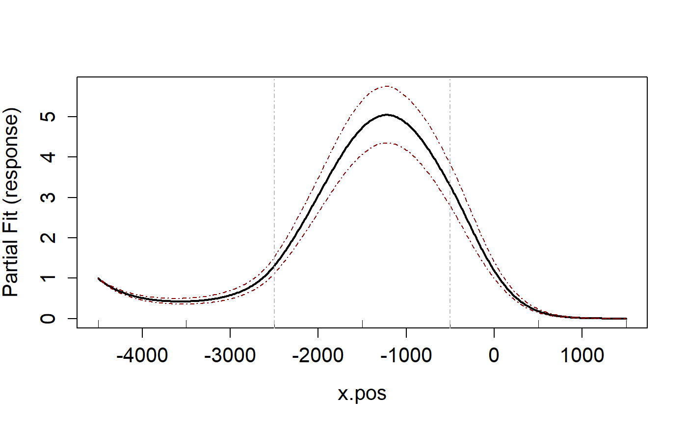

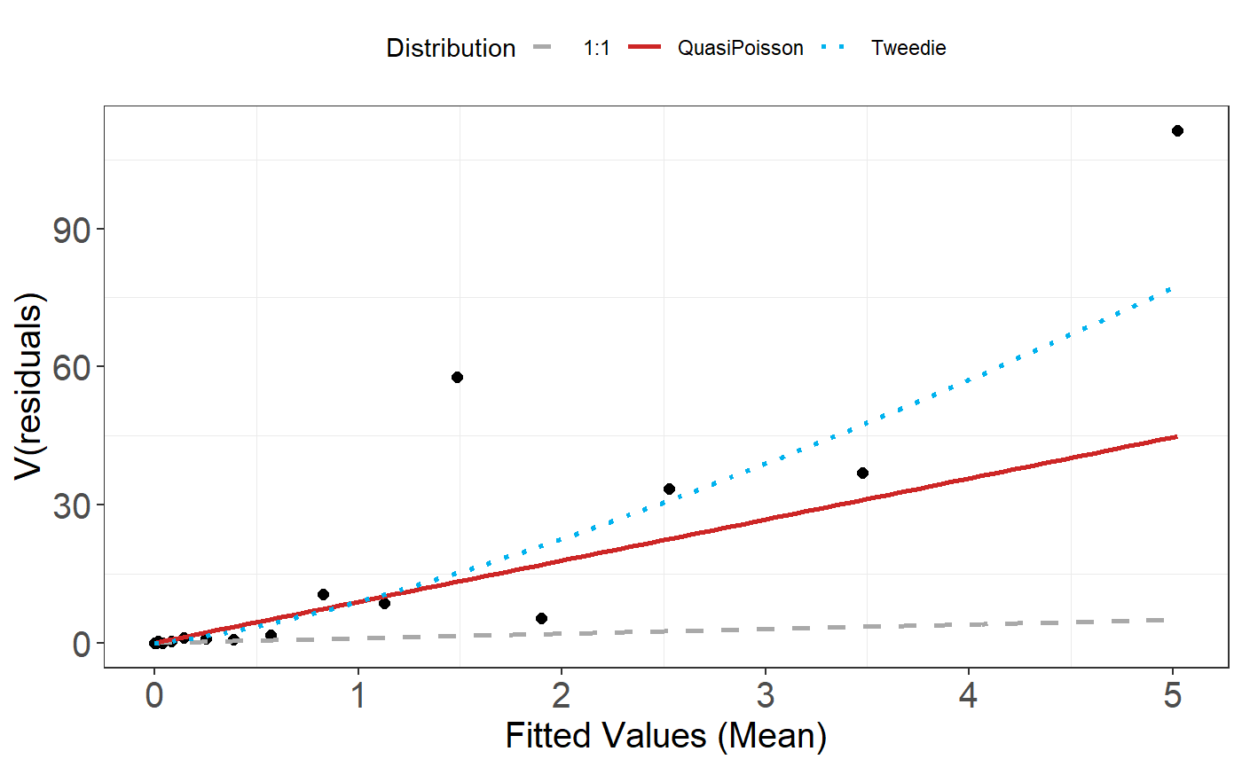
plotMeanVar(salsa1dOutput$bestModel)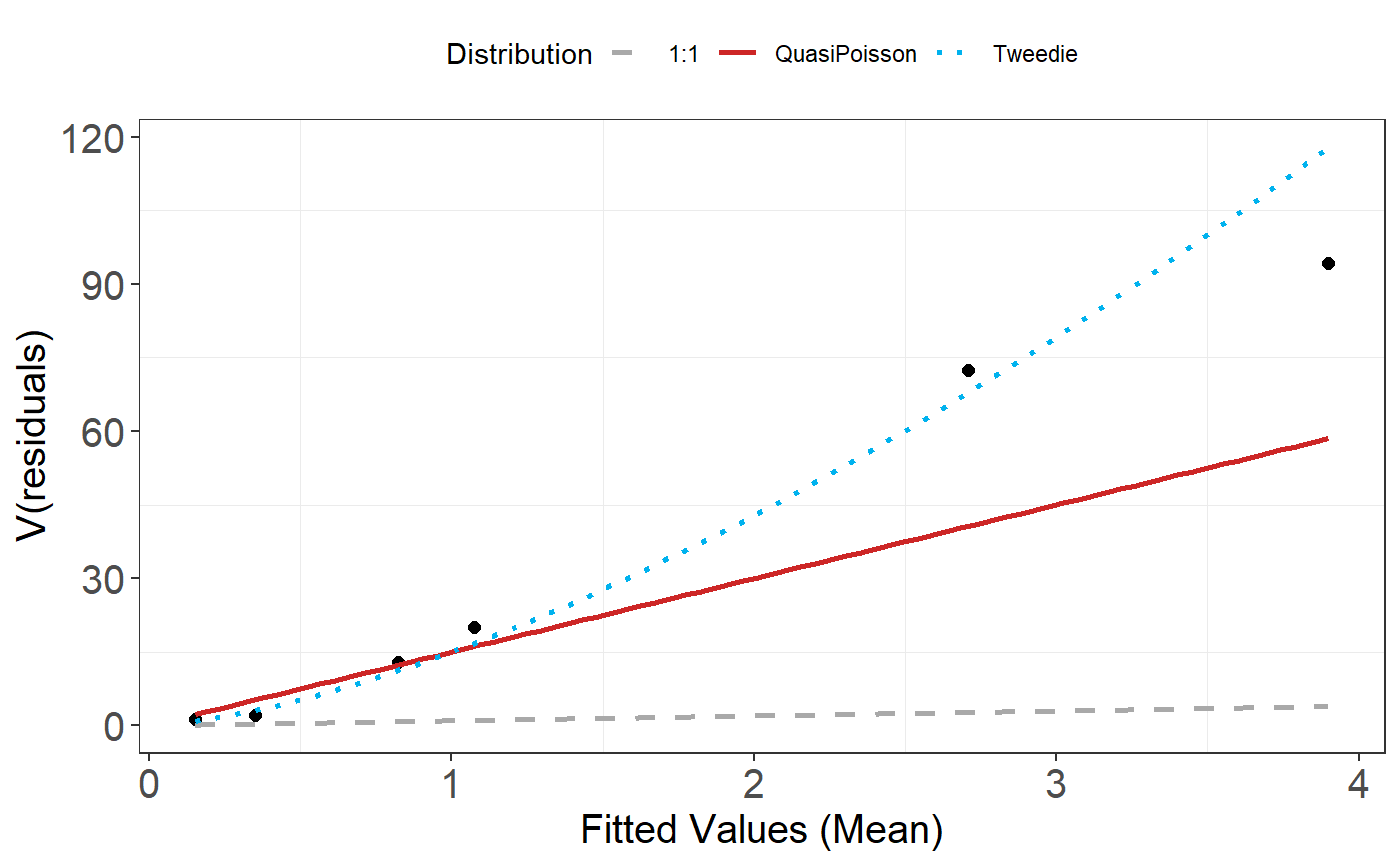

Two dimensional Smoothing

Starting point

This is the same starting point for one dimensional splines if it is only a two dimensional smooth you want.

Load some data
Fit an initial model. For simplicity we fit an intercept only model.

# load data
baselinedata <- filter(nysted.analysisdata, impact == 1, season == 1)

profout <- tweedie.profile(response ~ x.pos + y.pos + depth, 
                           data=baselinedata,
                           xi.vec = seq(1.01, 1.99, by=0.05), do.plot=TRUE)
#> 1.01 1.06 1.11 1.16 1.21 1.26 1.31 1.36 1.41 1.46 1.51 1.56 1.61 1.66 1.71 1.76 1.81 1.86 1.91 1.96 
#> ....................Done.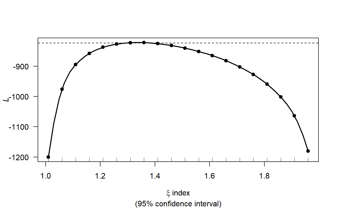

initialModel<- glm(response ~ 1, family=tweedie(var.power=profout$xi.max, link.power = 0),data=baselinedata)

kg <- getKnotgrid(baselinedata[, c("x.pos", "y.pos")], numKnots = 300, plot = FALSE)

# make distance matrices for datatoknots and knottoknots
distMats<-makeDists(baselinedata[, c("x.pos", "y.pos")], kg)

# make prediction distance matrix. 
preddata <- filter(nysted.predictdata, impact == 0, season == 1)
p2k <-makeDists(preddata[, c("x.pos", "y.pos")], kg, knotmat = FALSE)$dataDist

# make parameter set for running salsa2D
salsa2dlist<-list(fitnessMeasure = 'AICtweedie', 
                  knotgrid = na.omit(kg),
                  startKnots=10, 
                  minKnots=2, 
                  maxKnots=20, 
                  gap=0)

salsa2dOutput<-runSALSA2D(initialModel,
                          salsa2dlist, 
                          d2k=distMats$dataDist,
                          k2k=distMats$knotDist,
                          basis = "gaussian", ##
                          suppress.printout = TRUE)

preddata$preds.g <- predict(object = salsa2dOutput$bestModel, 
                            newdata = preddata, g2k = p2k)

ggplot() +
  geom_tile(data=preddata, aes(x.pos, y.pos, fill=preds.g, 
                               height=sqrt(area), width=sqrt(area))) + 
  xlab("Easting (km)") + ylab("Northing (km)") + coord_equal() +
  theme_bw() + ggtitle("Gaussian Basis") +
  scale_fill_distiller(palette = "Spectral",name="Animal Counts")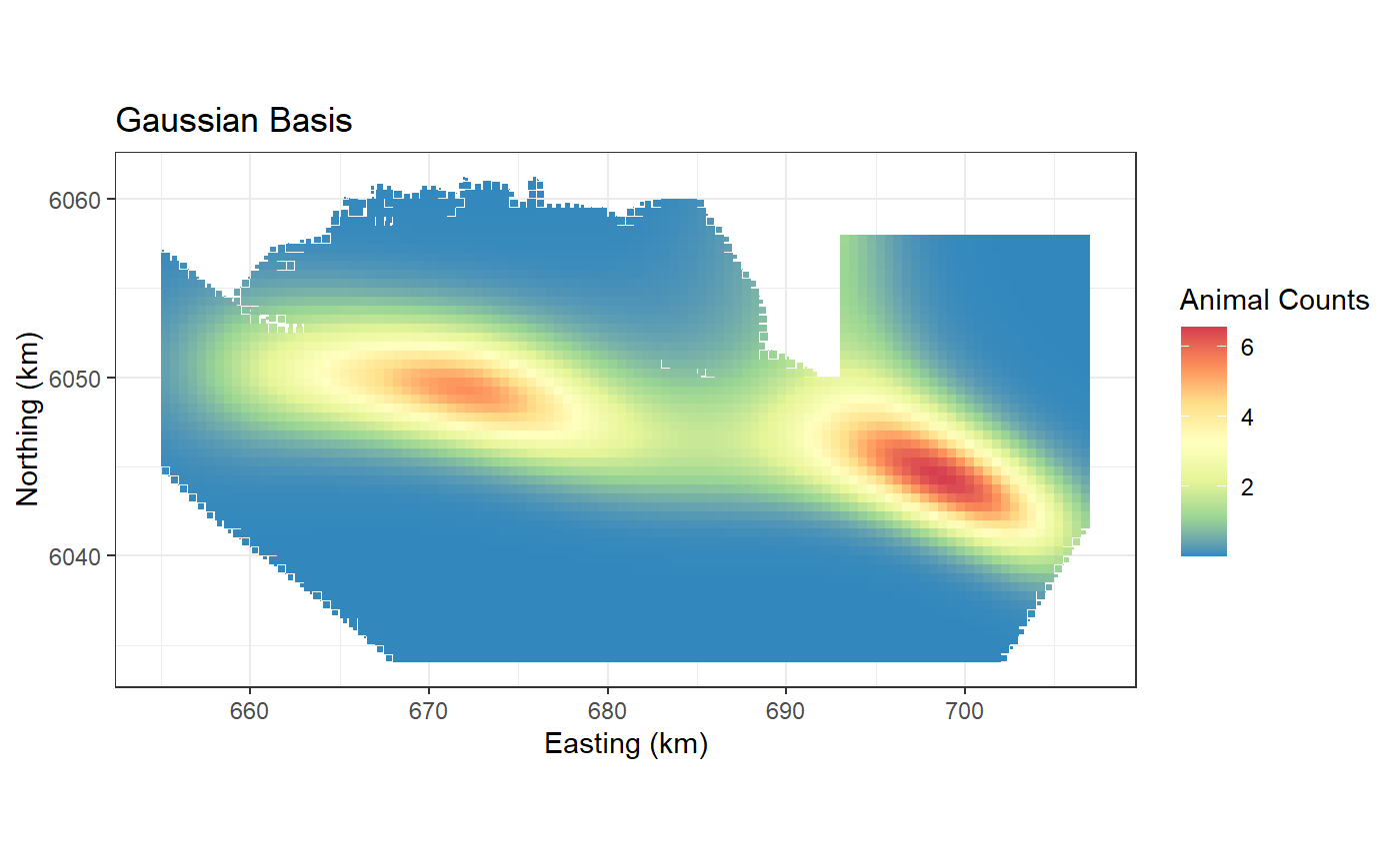

plotMeanVar(salsa2dOutput$bestModel)

Raw data for reference

ggplot() +
     geom_tile(data=baselinedata, aes(x.pos, y.pos, fill=response, height=sqrt(area), width=sqrt(area))) + 
     xlab("Easting (km)") + ylab("Northing (km)") + coord_equal() +
     theme_bw() + ggtitle("Raw Data") +
     scale_fill_distiller(palette = "Spectral",name="Animal Counts")

Lindesay Scott-Hayward

2024-05-08

The Tweedie distribution

An example of fitting the tweedie distribution in `R`

Setup

Fitting a `gamMRSea` model

Two dimensional Smoothing

Starting point

Raw data for reference

Using the Tweedie Distribution

Lindesay Scott-Hayward

2024-05-08

The Tweedie distribution

An example of fitting the tweedie distribution in R

Setup

Fitting a gamMRSea model

Two dimensional Smoothing

Starting point

Raw data for reference

An example of fitting the tweedie distribution in `R`

Fitting a `gamMRSea` model