MRSea: Marine Renewables Strategic Environmental Assessment
Lindesay Scott-Hayward
2023-08-30
Source:vignettes/web/IntroductiontoMRSea.Rmd
IntroductiontoMRSea.RmdIntroduction
MRSea stands for Marine Renewables Strategic
Environmental Assessment. and the package was developed for analysing
data that was collected for assessing potential impacts of renewable
developments on marine wildlife, although the methods are applicable to
any studies where you wish to fit uni or bivariate smooths.
The package enables the fitting of spatially adaptive regression splines using two Spatially Adaptive Local Smoothing Algorithms (SALSA):
- Generalised additive model framework using exponential family distributions (e.g. Gaussian, Poisson, Binomial, Gamma) and the Tweedie distribution.
- Univariate smoothing using B-splines, Natural cubic splines or cyclic cubic splines
- Bivariate smoothing using Gaussian or exponential radial basis functions
- Euclidean or geodesic distance metric for similarity between 2D points (distance component of the radial basis functions)
- Direct estimation of robust standard errors in the case of residual correlation
- Additionally there are development versions for point process and multinomial responses
For additional information regarding the methods see the Publications Page
The main modelling functions are runSALSA1D and
runSALSA2D, which implement the methods for univariate and
then bivariate smoothing and these produce models of the class
gamMRSea.
Other functions include diagnostics (to assess residual correlation:
runACF, smooth relationships: runPartialPlots
and model selection (ANOVA) for robust standard errors:
anova.gamMRSea) and inference
(do.bootstrap.cress).
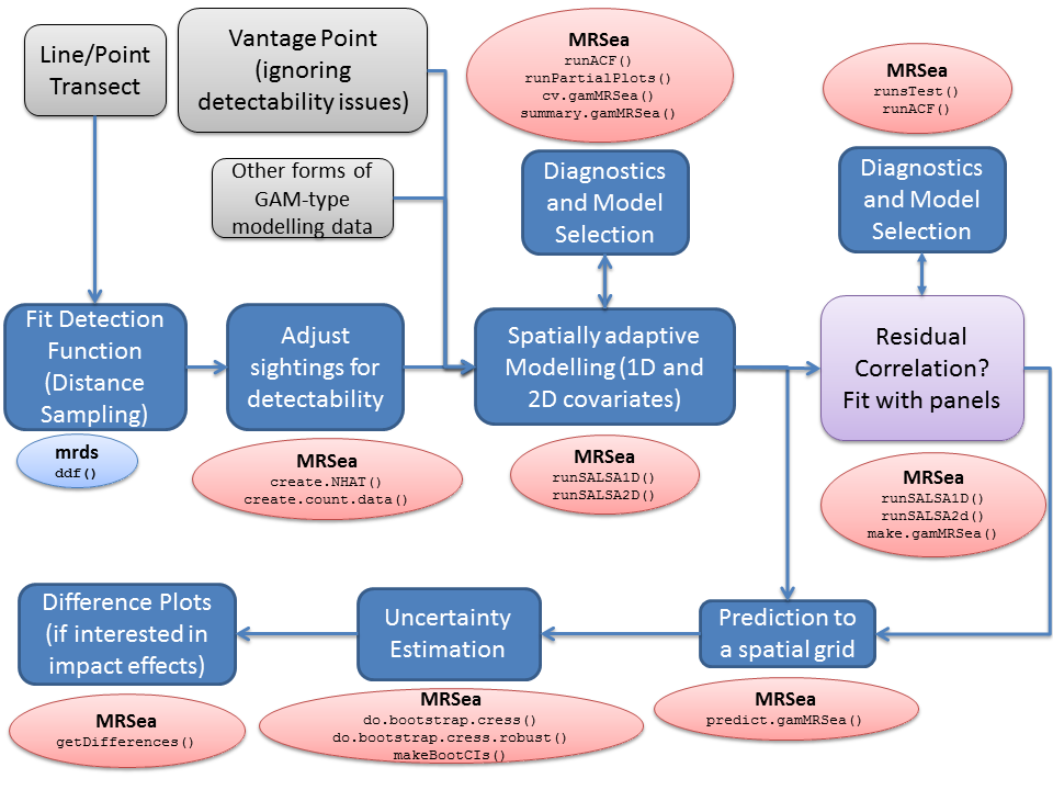 Example of the
modelling process using
Example of the
modelling process using MRSea. Packages with functions to
run certain parts are given in oval boxes. To complete the modelling
process, other packages may be used at certain stages. These are coded
light blue, whilst MRSea functions are in red.
Examples and tutorials on the MRSea Website
For information on using the package see here for a list of examples and tutorials.
Translating from glm to gamMRSea
Making any glm model into an gamMRSea
object
This can be done using the make.gamMRSea function. Here
we use the fullmodel which is a glm model with
family='poisson'
library(MRSea)
data("nysted.analysisdata")
fit <- glm(response ~ season + depth, family="quasipoisson", data = nysted.analysisdata)
fullModel.gamMRSea <- make.gamMRSea(fit,
                                    gamMRSea = TRUE)
summary(fullModel.gamMRSea)
#>
#> Call:
#> gamMRSea(formula = response ~ season + depth, family = "quasipoisson",
#>     data = nysted.analysisdata)
#>
#> Deviance Residuals:
#>     Min       1Q   Median       3Q      Max
#> -1.9124  -1.0821  -0.7745  -0.5392  20.9195
#>
#> Coefficients:
#>              Estimate Std. Error Robust S.E. t value Pr(>|t|)
#> (Intercept)  0.995330   0.131116    0.131116   7.591 3.48e-14 ***
#> season      -0.352263   0.048872    0.048872  -7.208 6.13e-13 ***
#> depth        0.096207   0.008387    0.008387  11.470  < 2e-16 ***
#> ---
#> Signif. codes:  0 '***' 0.001 '**' 0.01 '*' 0.05 '.' 0.1 ' ' 1
#>
#> (Dispersion parameter for quasipoisson family taken to be 11.58097)
#>
#>     Null deviance: 26118  on 9231  degrees of freedom
#> Residual deviance: 23676  on 9229  degrees of freedom
#> AIC:  NA
#>
#> Max Panel Size = 1 (independence assumed); Number of panels = 9232
#> Number of Fisher Scoring iterations: 7
Note that there is an extra column for robust standard errors but
that they are the same as the raw ones. No panel structure has been
specified and this is shown at the bottom of the output
Max Panel Size = 1.
Adding a panel structure to a model
Additionally, if you choose to fit the SALSA or GLM models without a
panel structure, the make.gamMRSea function can be used to
add a panel structure afterwards. Note that now in the summary output,
the robust standard error column is different to the raw standard errors
as they have been adjusted for any correlation seen in the panels. The
output shows that the maximum panel size is now 54 and there are 208
panels.
fit.robustse <- make.gamMRSea(fit,
                              gamMRSea = TRUE,
                              panelid = nysted.analysisdata$transect.id)
summary(fit.robustse)
#>
#> Call:
#> gamMRSea(formula = response ~ season + depth, family = "quasipoisson",
#>     data = nysted.analysisdata)
#>
#> Deviance Residuals:
#>     Min       1Q   Median       3Q      Max
#> -1.9124  -1.0821  -0.7745  -0.5392  20.9195
#>
#> Coefficients:
#>              Estimate Std. Error Robust S.E. t value Pr(>|t|)
#> (Intercept)  0.995330   0.131116    0.177209   5.617 2.00e-08 ***
#> season      -0.352263   0.048872    0.071747  -4.910 9.27e-07 ***
#> depth        0.096207   0.008387    0.004515  21.310  < 2e-16 ***
#> ---
#> Signif. codes:  0 '***' 0.001 '**' 0.01 '*' 0.05 '.' 0.1 ' ' 1
#>
#> (Dispersion parameter for quasipoisson family taken to be 11.58097)
#>
#>     Null deviance: 26118  on 9231  degrees of freedom
#> Residual deviance: 23676  on 9229  degrees of freedom
#> AIC:  NA
#>
#> Max Panel Size = 54; Number of panels = 208
#> Number of Fisher Scoring iterations: 7